
DAGs and Confounding Part II -- Simultaneity Bias
In this second installment on DAGs and confounding, I’m cheating, slightly. The name Directed Acyclic Graph implies no cycles and unidirectional causal paths in a set of causal relationships. However, in many settings, we may encounter forms of confounding that are indeed cyclical and multidirectional. I’m referring specifically to simultaneity bias—a form of endogeneity introduced through mutual causation of two or more variables.
In this post I want to briefly walk through a connonical example (at least a Google search would suggest it is as much), how to illustrate it via a DAG-like framework (remember these won’t be true DAGs since the causal relations violate the D and A parts of the acronym), and a simulation to illustrate the bias it introduces and how we can get around it.
What is simultaneity bias?
There are many forms of endogeneity that may exist in data. One such form is simultaneity—a scenario where two outcomes are mutually causal. Such a scenario is depicted in the figure below.
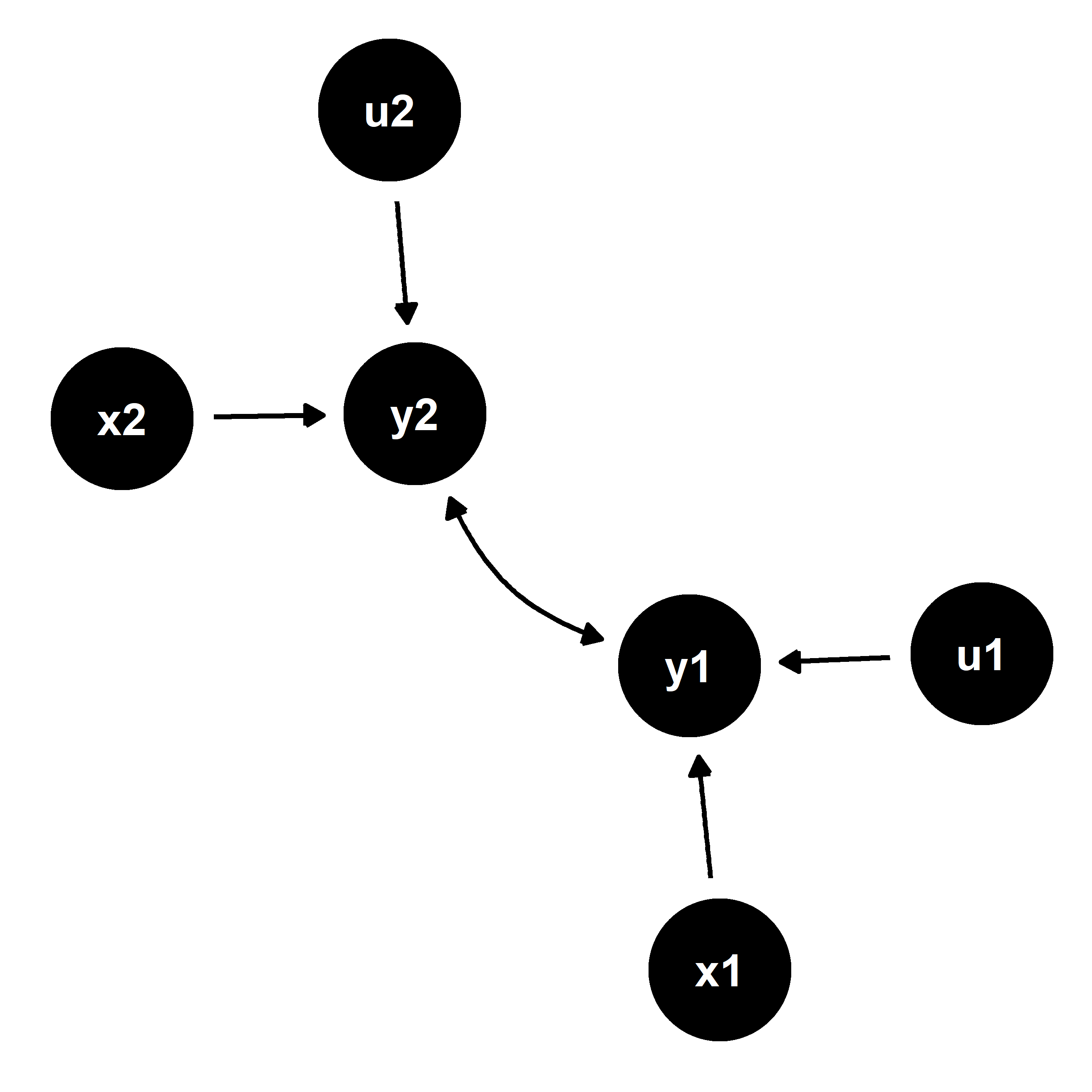
We have two endogenous outcomes of interest, y1 and y2. These are a function of a set of observed exogenous outcomes, x1 and x2 respectively, and some unobserved exogenous variables, u1 and u2.
Within a regression framework, such an instance can be represented as a structural equation. For example:
y1 = α1y2 + α2x1 + u1,
y2 = β1y1 + β2x2 + u2,
where y1 and y2 are the endogenous outcomes, x1 and x2 are exogenous predictors, and u1 and u2 are unobserved predictors—and thus random noise.
Under only very restrictive assumptions can we reliably estimate such a system of equations using OLS. If α1 and β1 are non-zero—as they would be if y1 and y2 are endogenous—OLS estimates will be biased and inefficient. The reason for this can be seen by expressing these equations in reduced form. For example, for y1:
y1 = α1y2 + α2x1 + u1,
y1 = α1(β1y1 + β2x2 + u2) + α2x1 + u1,
y1(1 − α1β1) = α1β2x2 + α2x1 + α1u2 + u1,
y1 = π1x2 + π2x1 + v1,
where the reduced form parameters are nonlinear functions of the structural parameters:
π1 = α1β2/(1 − α1β1);
π2 = α2/(1 − α1β1);
v1 = (α1u2 + u1)/(1 − α1β1).
There is a similar reduced form equation for y2. We’ll denote it as:
y2 = γ1x1 + γ2x2 + v2.
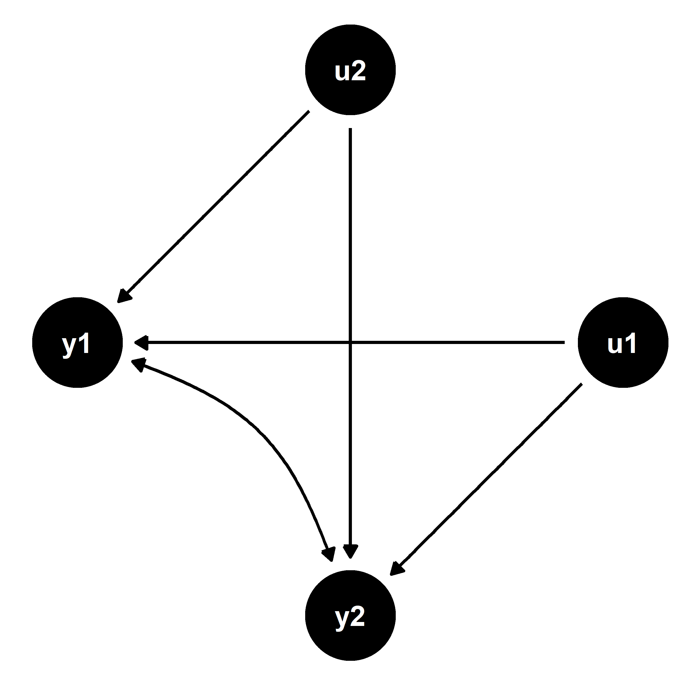
From this formulation we can see in the construction of the new error terms v1 and v2 that y1 will be correlated with the error term through y1’s correlation with u2—and y2 will be correlated with the error term through its correlation with u1. This is problematic for the estimation of the structural equations via OLS because it means that in estimating the regression for y1, the unobserved variation captured by u1 confounds the relationship between y1 and y2—the same is true for u2 in the second regression equation.
The below figure illustrates for clarity. Though it was not immediately apparent in the first figure, the causal relationships it represents imply the confounding captured in this one.
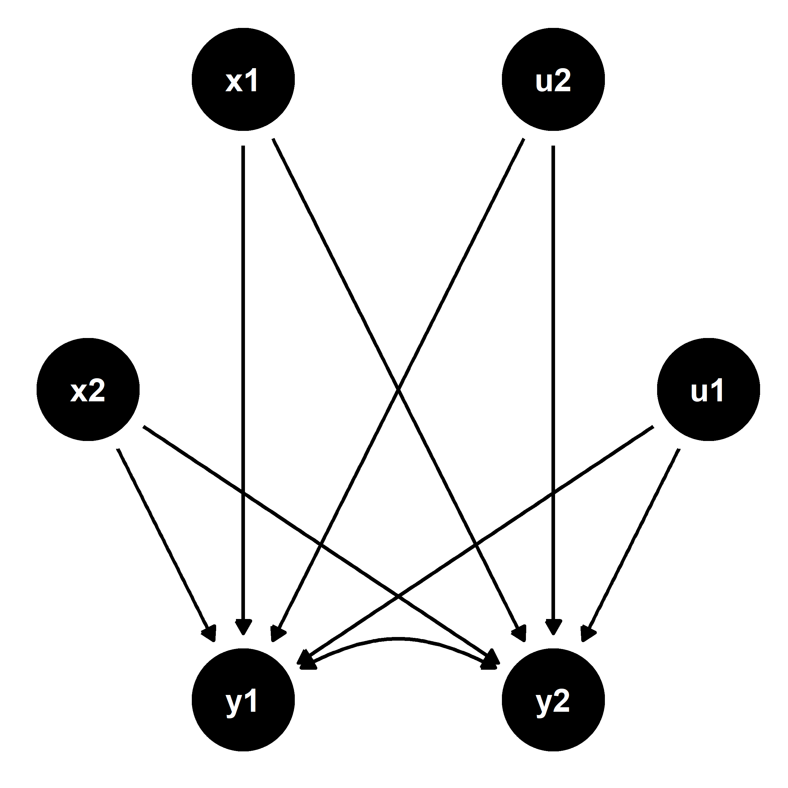
Because u1 and u2 are unobserved, we cannot control for them in order to reliably estimate the effect of y1 on y2, and vice versa. However, it is possible to reliably estimate the reduced form equations since the error terms are not correlated with the exogenous predictors x1 and x2. This is illustrated by the next figure below and can be leveraged to recover unbiased estimates of the causal relationships between the endogenous outcomes.
To demonstrate, I’ve simulated a data generating process as follows
using tools from the seerrr package, with the structural parameters
defined each as 1/2:
# Structural parameters:
a1 <- 0.5
a2 <- 0.5
b1 <- 0.5
b2 <- 0.5

# Reduced form:
p1 <- (a1 * b1) / (1 - a1 * b1)
p2 <- a2 / (1 - a1 * b1)
q1 <- (b1 * a1) / (1 - b1 * a1)
q2 <- a1 / (1 - b1 * a1)

# Simulate the d.g.p.
simulate(
  u1 = rnorm(N),
  u2 = rnorm(N),
  x1 = rnorm(N),
  x2 = rnorm(N),
  y1 = p1 * x2 + p2 * x1 + (a1 * u2 + u1) / (1 - a1 * b1),
  y2 = q1 * x1 + q2 * x2 + (a2 * u1 + u2) / (1 - b1 * a1)
) -> sim_dat
By default, this generates a list of 200 datasets drawn from the data generating process where N = 500. Using multiple draws from the d.g.p. in this way allows us to get a sense for how generally reliable estimates of the parameters are. Because we’re dealing with random variables, some variation in performance from sample to sample is expected.
With these draws, I estimate a distribution of OLS estimates for the reduced form equations:
estimate(
  sim_dat,
  y1 ~ x2 + x1,
  c("x1", "x2"),
  se_type = "stata"
) -> red1
estimate(
  sim_dat,
  y2 ~ x1 + x2,
  c("x1", "x2"),
  se_type = "stata"
) -> red2
And for the structural equations:
estimate(
  sim_dat,
  y1 ~ y2 + x1,
  c("y2", "x1"),
  se_type = "stata"
) -> str1
estimate(
  sim_dat,
  y2 ~ y1 + x2,
  c("y1", "x2"),
  se_type = "stata"
) -> str2
Next, I evaluate the bias in the reduced form estimates:
bind_rows(
  evaluate(
    red1 %>% filter(term == "x2"),
    what = "bias",
    truth = p1
  ) %>% mutate(param = "pi[1]"),
  evaluate(
    red1 %>% filter(term == "x1"),
    what = "bias",
    truth = p2
  ) %>% mutate(param = "pi[2]")
) -> red_bias1
bind_rows(
  evaluate(
    red2 %>% filter(term == "x1"),
    what = "bias",
    truth = q1
  ) %>% mutate(param = "gamma[1]"),
  evaluate(
    red2 %>% filter(term == "x2"),
    what = "bias",
    truth = q2
  ) %>% mutate(param = "gamma[2]")
) -> red_bias2
And for the structural equation estimates:
bind_rows(
  evaluate(
    str1 %>% filter(term == "y2"),
    what = "bias",
    truth = a1
  ) %>% mutate(param = "alpha[1]"),
  evaluate(
    str1 %>% filter(term == "x1"),
    what = "bias",
    truth = a2
  ) %>% mutate(param = "alpha[2]")
) -> str_bias1
bind_rows(
  evaluate(
    str2 %>% filter(term == "y1"),
    what = "bias",
    truth = b1
  ) %>% mutate(param = "beta[1]"),
  evaluate(
    str2 %>% filter(term == "x2"),
    what = "bias",
    truth = b2
  ) %>% mutate(param = "beta[2]")
) -> str_bias2
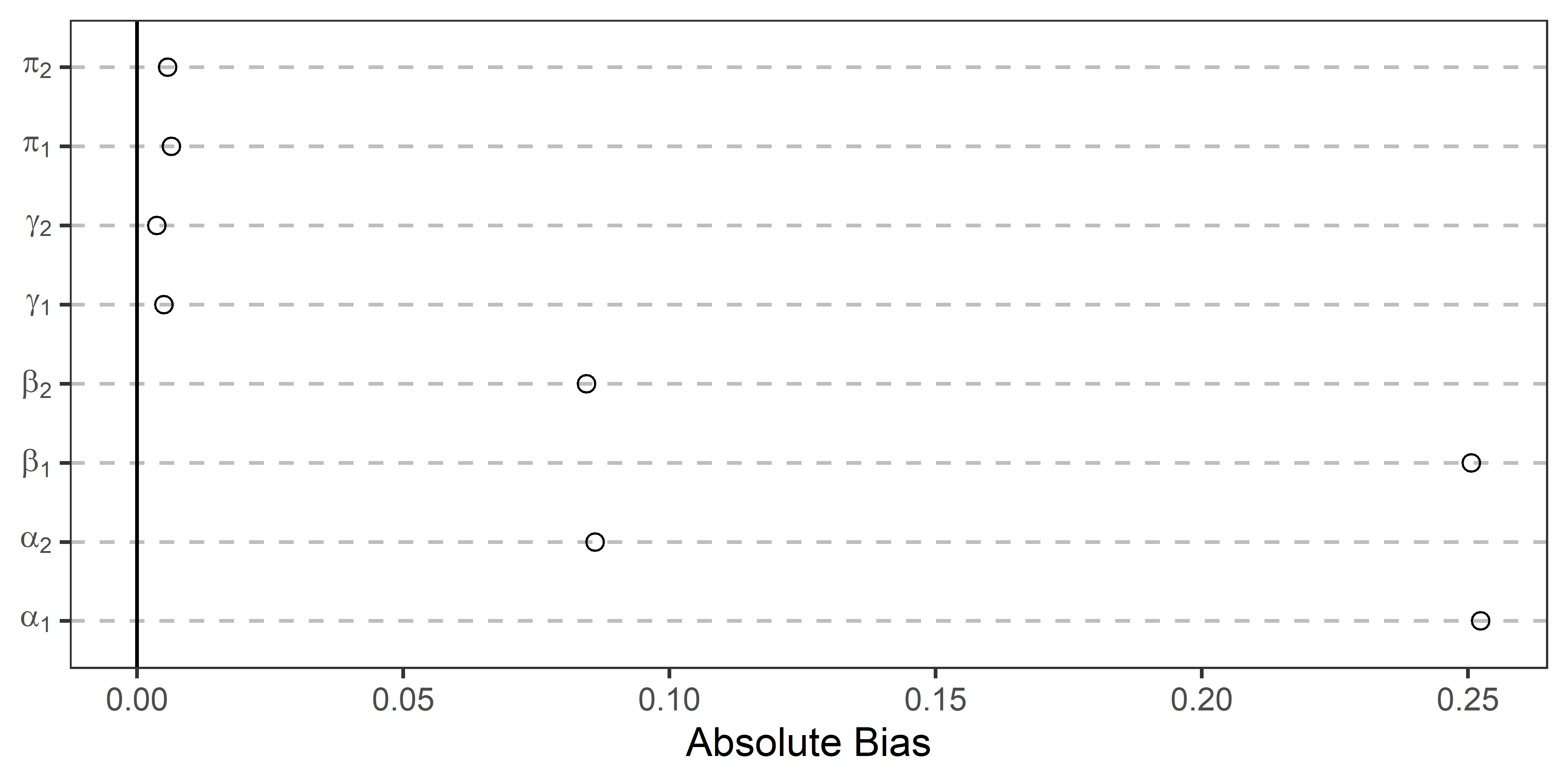
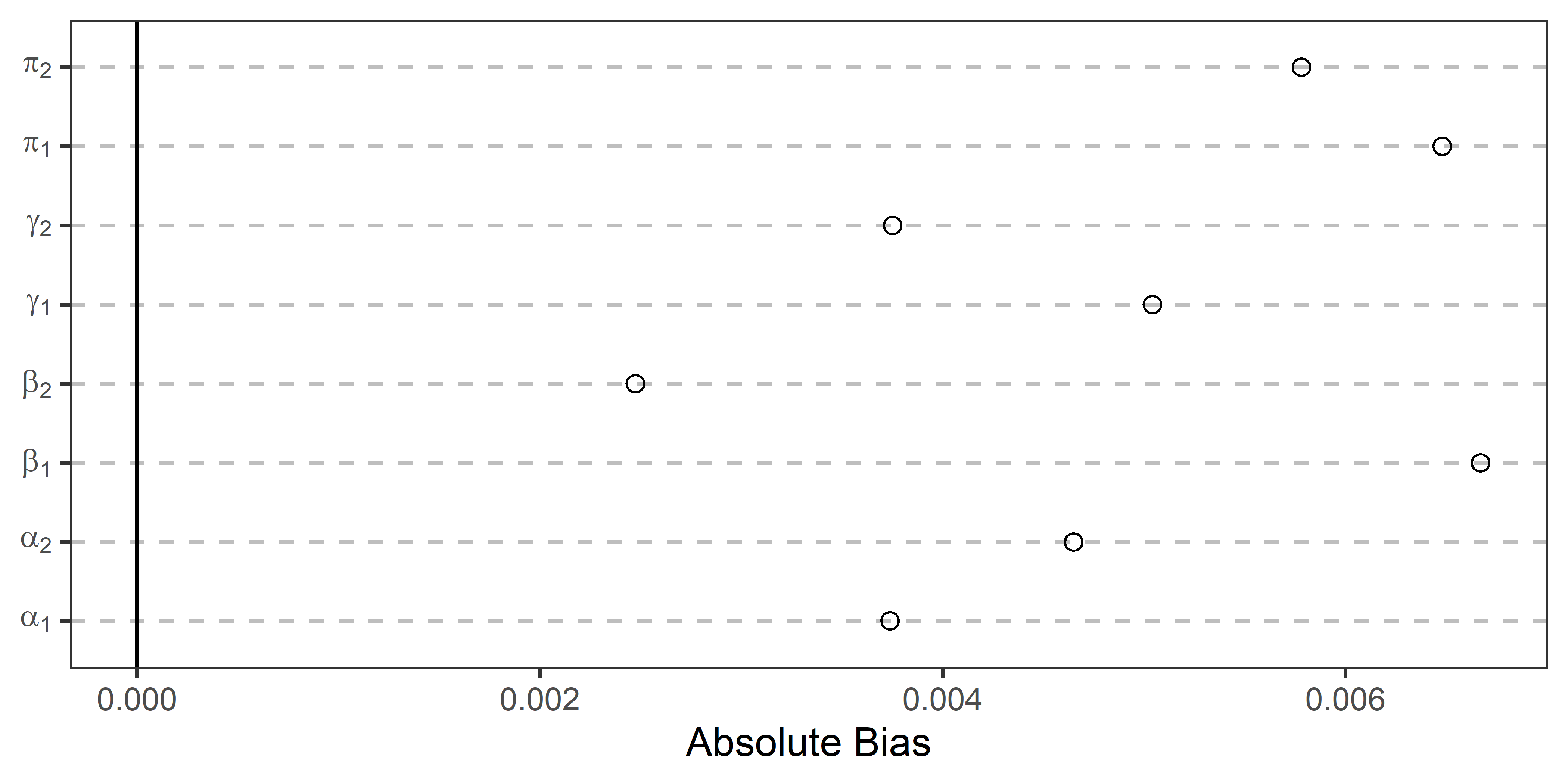
The below figure shows the results for each of the parameters. The absolute average bias is given along the x-axis and the relevant parameter is indicated along the y-axis. If the point estimate is closer to zero the closer the average estimate is to its true value. By this metric, the systematic bias in the structural parameter estimates is quite evident.
What can be done?
Clearly the reduced form specification is more consistent. However, in practice the reduced form estimates, while reliable, are not as informative as we would like. More often the structural parameters are of greatest theoretical interest. So how can we reliably recover these?
One option is an instrumental variables (IV) approach. This is usually done via two-stage least squares (TSLS). This entails using the reduced form equations in a first-stage regression for each of the outcomes, then using the fitted outcomes from the reduced form equations as predictors in the structural equations in the second stage. E.g.:
- Stage 1—estimate the reduced form equations:
y1 = π1x2 + π2x1 + v1,
y2 = γ1x1 + γ2x2 + v2.
- Stage 2—use predictions from stage 1 as regressors in stage 2:
y1 = α1ŷ2 + α2x1 + u1,
y2 = β1ŷ1 + β2x2 + u2.
This approach works for generating reliable estimates of the structural parameters in the second stage because the fitted values of y1 and y2 on the right-hand side of the equations are no longer correlated with the error terms. This removes the unobserved confounding captured by u1 and u2.
I first apply the IV approach on our simulated data:
estimate(
  sim_dat,
  y1 ~ y2 + x1 | x2 + x1,
  c("y2", "x1"),
  se_type = "stata",
  estimator = iv_robust
) -> tsls1
estimate(
  sim_dat,
  y2 ~ y1 + x2 | x2 + x1,
  c("y1", "x2"),
  se_type = "stata",
  estimator = iv_robust
) -> tsls2
I then calculate average bias:
bind_rows(
  evaluate(
    tsls1 %>% filter(term == "y2"),
    what = "bias",
    truth = a1
  ) %>% mutate(param = "alpha[1]"),
  evaluate(
    tsls1 %>% filter(term == "x1"),
    what = "bias",
    truth = a2
  ) %>% mutate(param = "alpha[2]")
) -> tsls_bias1
bind_rows(
  evaluate(
    tsls2 %>% filter(term == "y1"),
    what = "bias",
    truth = b1
  ) %>% mutate(param = "beta[1]"),
  evaluate(
    tsls2 %>% filter(term == "x2"),
    what = "bias",
    truth = b2
  ) %>% mutate(param = "beta[2]")
) -> tsls_bias2
The results are shown below. Again these are depicted relative to the average bias of the reduced form parameters. Note the difference relative to before. The estimates of the structural parameters have substantially reduced bias—practically performing just as well as the reduced form parameter estimates.
Conclusion
So that concludes Part II of this series. Check out the last post for a discussion of another type of bias (post treatment bias), and see here for a discussion of endogeneity.