
DAGs and Confounding Part I
Directed acyclic graphs (DAGs) help in visualizing causal relationships among variables. But, I have to admit, making sense of DAGs and what the relationships they represent imply for empirical analysis is not always easy.
In this first installment of what will be a series of posts, I want to illustrate how relationships captured by DAGs impact analytical choices in empirical analysis. I do this with some simple simulations.
In this post I kick things off with a focus on post-treatment bias.
Post Treatment and d-connectedness
Suppose three variables, x, y, and z. Say z → x and z → y (where → represents a causal relationship). I’ve captured this relationship in the DAG below:
library(tidyverse)
library(seerrr)
library(ggdag)
theme_set(theme_dag())
confounder_triangle() %>%
  ggdag()
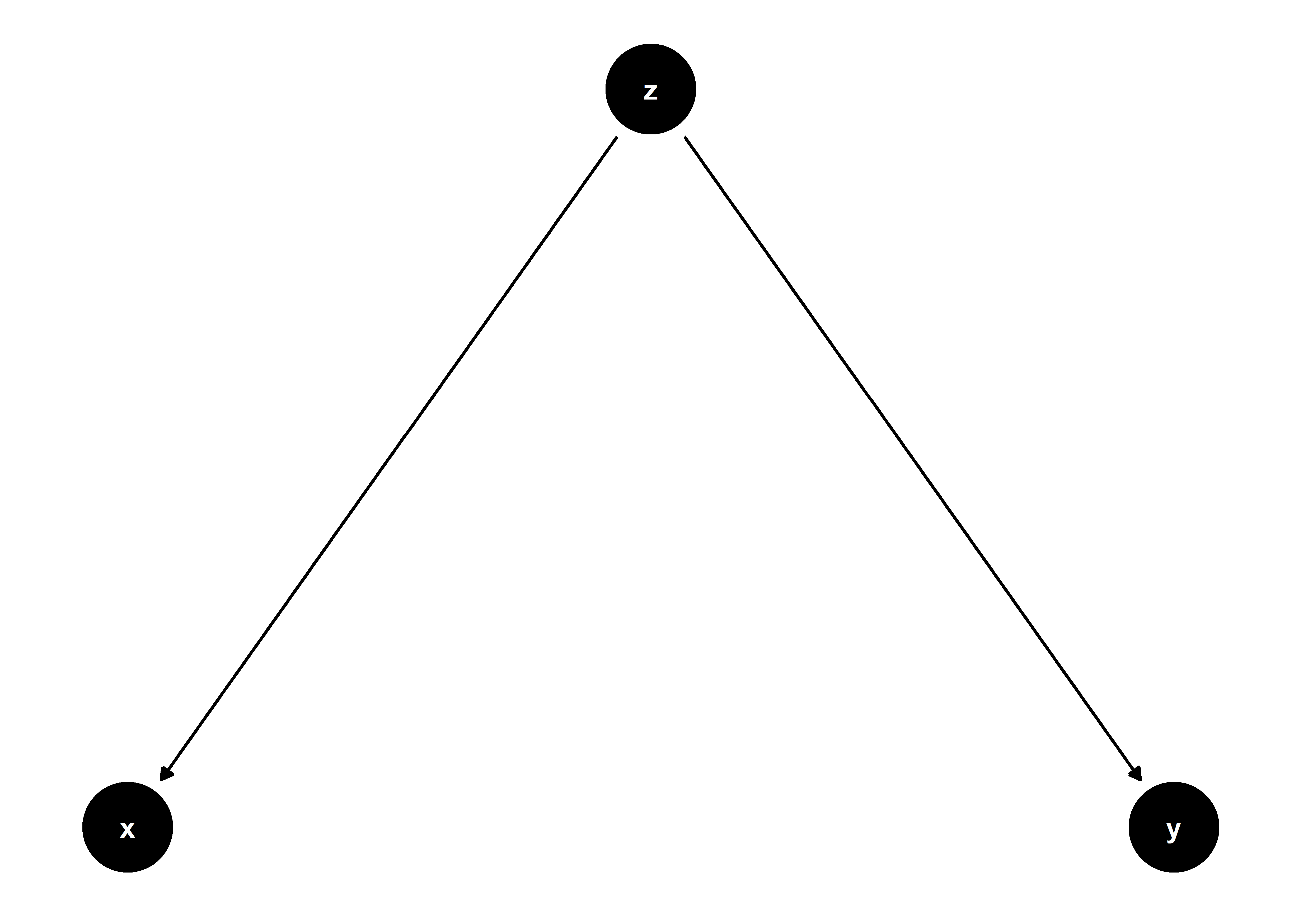
Suppose we want to recover an estimate of z’s effect on y. If we want an unbiased and efficient estimate (why wouldn’t we?) it would be inappropriate to control for x in our analysis.
Why? x and y are “d-connected,” (directional connected) as highlighted the below updated DAG:
confounder_triangle() %>%
  ggdag_dconnected()
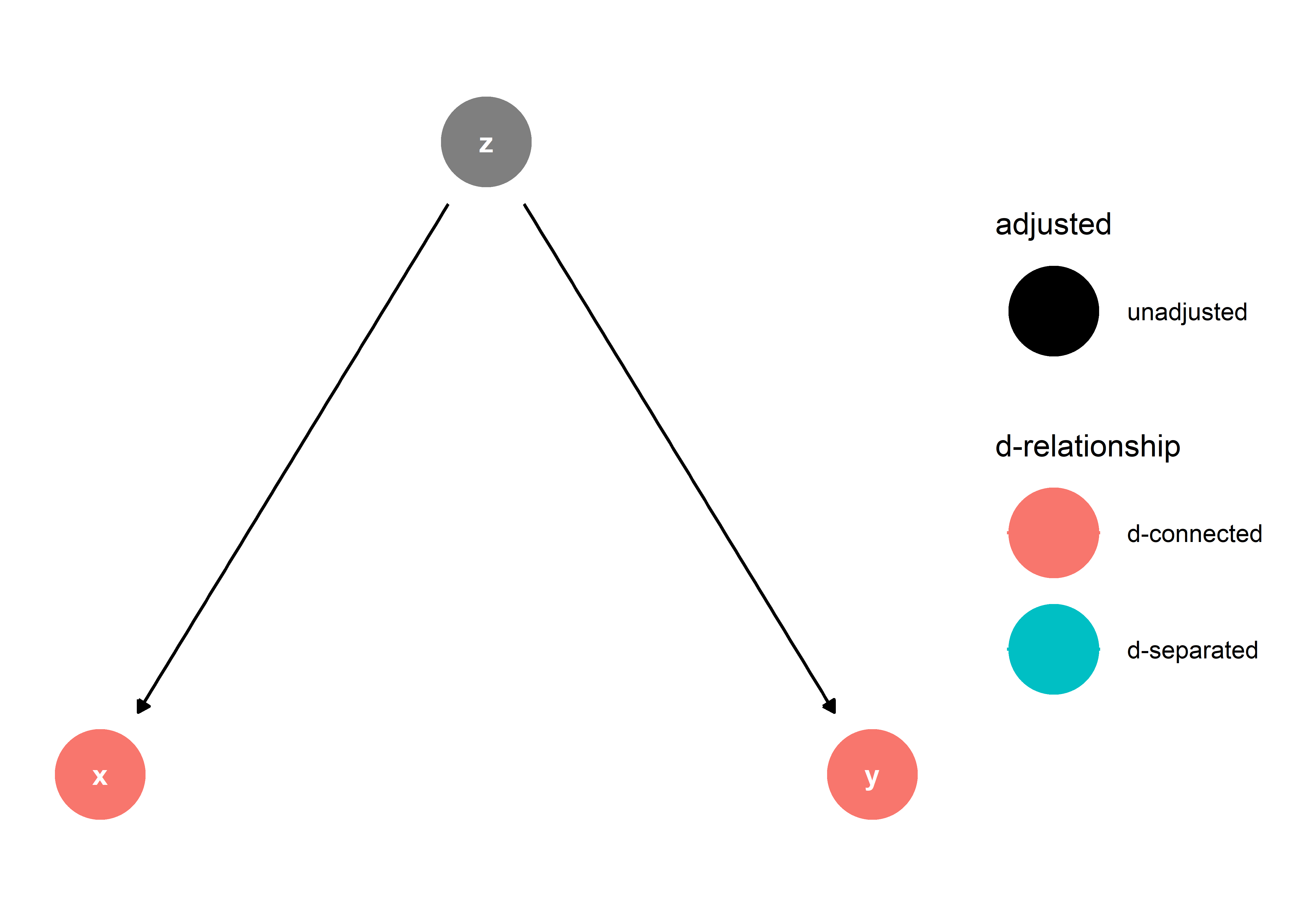
This means that x and y are related to each other due to their mutual cause, z. Such a relationship does not need to be accounted for in estimating the effect of z on y. In fact, if we were to adjust for x in our analysis, this would introduce a new type of relationship between x and y: that they are “d-separated”.
confounder_triangle() %>%
  ggdag_dconnected(
    controlling_for = "x"
  )
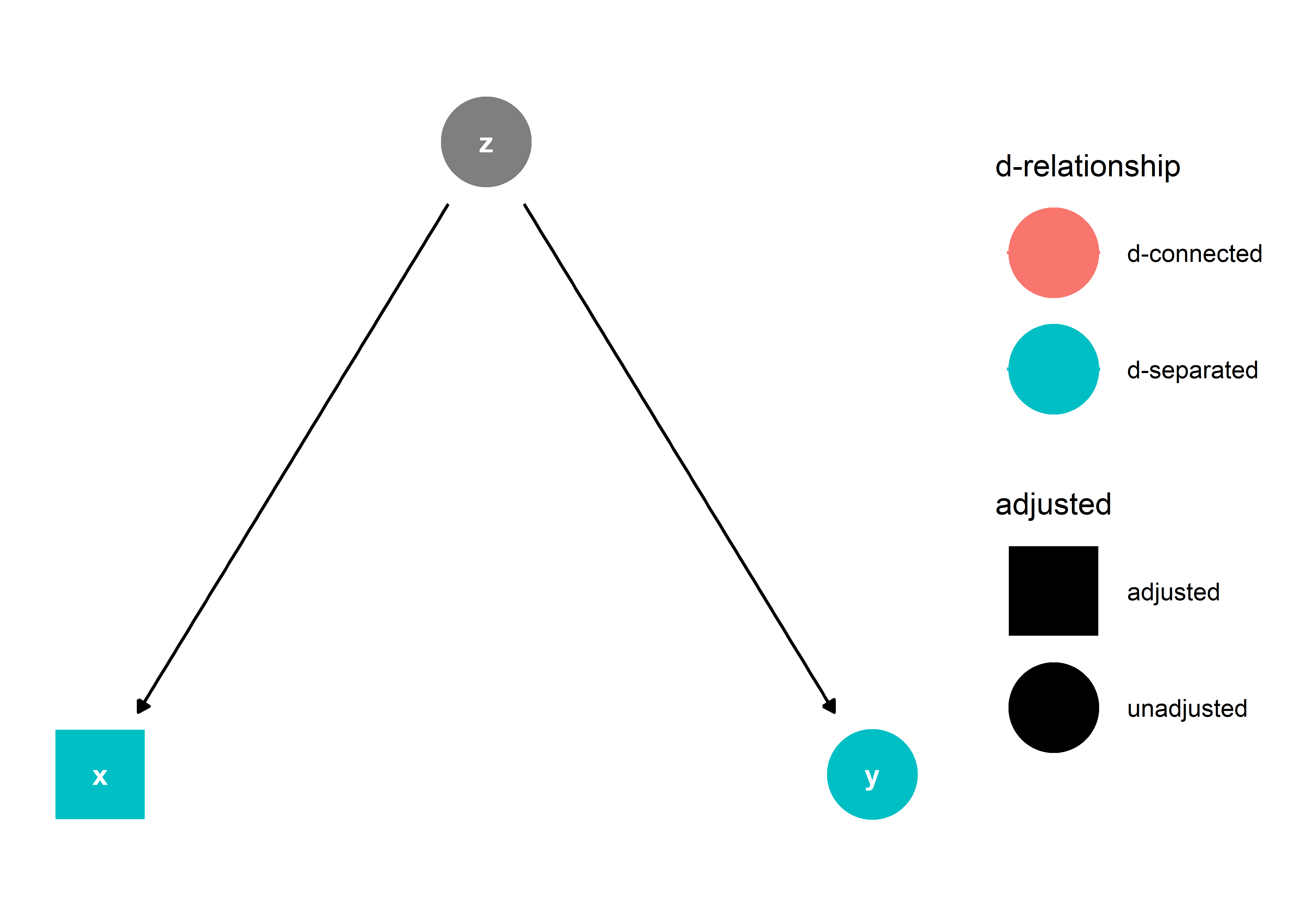
This is no good because we risk soaking up some of z’s effect on y by d-separating (yes, I’m using this as a verb) x and y. I’ll illustrate first with a simulation then try to provide some intuition for why this happens.
First, let’s simulate some data where there is a simple linear relationship between z and each of the effected variables, x and y:
set.seed(555)
simulate(
  R = 1000,
  N = 500,
  z = rnorm(N),
  y = z + rnorm(N),
  x = z + rnorm(N)
) -> sim_data
Next, let’s estimate the effect of z on y, both with and without adjusting for x:
# no adjustment for x:
estimate(
  sim_data,
  y ~ z,
  vars = "z",
  se_type = "stata"
) -> unadj

# with adjustment for x:
estimate(
  sim_data,
  y ~ z + x,
  vars = "z",
  se_type = "stata"
) -> adj
Now, let’s compare performance:
evaluate(
  unadj,
  what = "bias",
  truth = 1
) -> unadj_eval
evaluate(
  adj,
  what = "bias",
  truth = 1
) -> adj_eval
bind_rows(
  unadj_eval,
  adj_eval
) %>%
  mutate(
    method = c("unadjusted", "adjusted")
  ) %>%
  pivot_longer(
    cols = bias:mse
  ) %>%
  ggplot() +
  aes(
    x = value,
    y = method
  ) +
  facet_wrap(~ name) +
  geom_point() +
  geom_vline(
    xintercept = 0,
    lty = 2
  ) +
  theme_bw() +
  labs(
    x = "Estimate",
    y = NULL,
    title = "Adjusting for 'x' is no good!"
  )
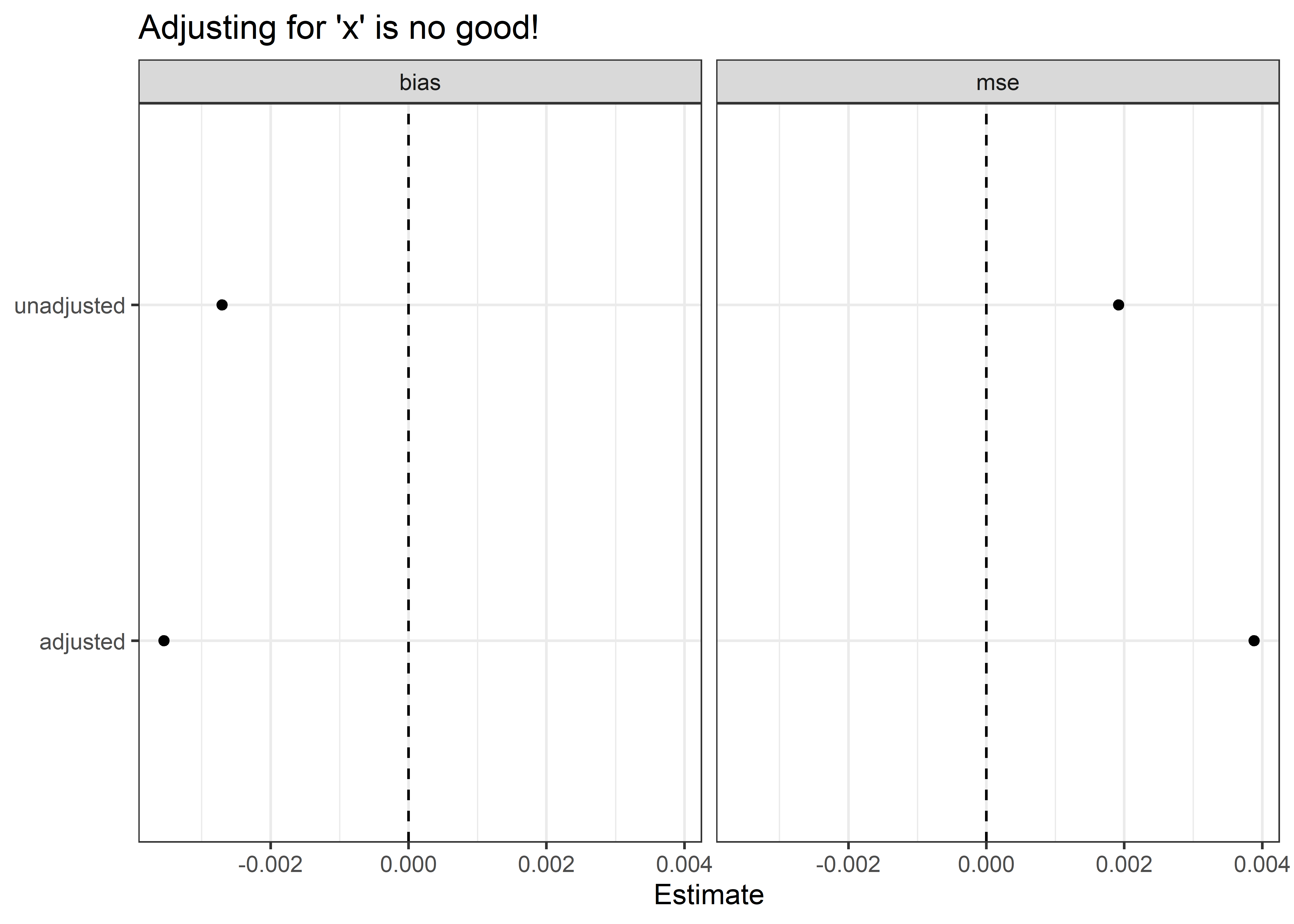
Controlling for x both worsens bias and efficiency. The reason for this is straightforward. In a regression model where y is regressed on both z and x
yi = β0 + β1zi + β2xi + εi,
the least squares solution for β1 is identified using variation in z not absorbed by x and variation in y not absorbed by x. This is problematic because we know that x has no direct effect on either of these variables. However, x does have a relationship with each since x is caused by z and shares a cause with y.
When we estimate a linear regression like that specified above using OLS, this is equivalent to performing three separate linear regressions. First, regressing z on x:
zi = α0 + α1xi + νi,
then regressing y on x:
yi = δ0 + δ1xi + μi,
and then finally regressing the residual variation in yi on zi:
μi = γ + β1νi + εi,
where the estimate for β1 here is equivalent to the one recovered from the multiple regression shown earlier.
This estimate will be incorrect because the identified relationships for the first two regression models will be biased. While there is no true effect of x on y, we nonetheless recover a relationship between them in the first regression:
estimate(
  sim_data,
  y ~ x,
  vars = "x",
  se_type = "stata"
) -> xy
mean(xy$estimate) # mean recovered estimate is > 0
## [1] 0.4982886
And, because z causes x, we recover a relationship between x and z from the second regression:
estimate(
  sim_data,
  z ~ x,
  vars = "x",
  se_type = "stata"
) -> xz
mean(xz$estimate) # mean recovered estimate is > 0
## [1] 0.4991261
Consequently, variation in z that causes x is subtracted out in the second regression—with some of the variation in z that causes y inevitably removed as well. Further, variation in y caused by z that also causes variation in x is removed in the first regression. This puts us at a clear disadvantage in estimating the effect of z on y.
A Simple Lesson
The lesson is simple. Do not control for post-treatment variables. This may seem obvious, but this is an issue that sometimes receives insufficient attention. Naturally, our instinct is to control for as many variables as possible in our analysis—especially in observational studies. But, as the case of post-treatment bias illustrates, this approach does not always serve us well.
This is where plotting out causal relationships with a DAG can be useful. By first thinking carefully and systematically about the relationships that exist in your data, it is possible to hedge against inappropriate analytical choices. DAGs, in short, can enhance your modeling instincts and ultimately serve to make you a better analyst.
There are other pitfalls beside post-treatment effects to be leery of, however. Next time we’ll take a look at another source of bias: colliders.