
Explaining Endogeneity and Instrumental Variables with seerrr
Building intuition for what endogeneity is and how instrumental variables (IV) help us deal with it is hard. I find that running a simulation helps me better grasp what the problem is, what it implies, and how IV helps.
To that end, tools in the seerrr package for R make devising, implementing, and summarizing such a simulation quite easy. So I’m using this post as an opportunity to do two things: (1) to provide some programmatic intuition for conceptualizing the problem of endogenous variables and (2) to put in a shameless plug for the convenience of using seerrr for doing this, and by extension, other simulation-based analyses.
Endogeneity
First, let’s address endogeneity. What is it?
This question is best answered by way of an illustration. Enter the DAG…
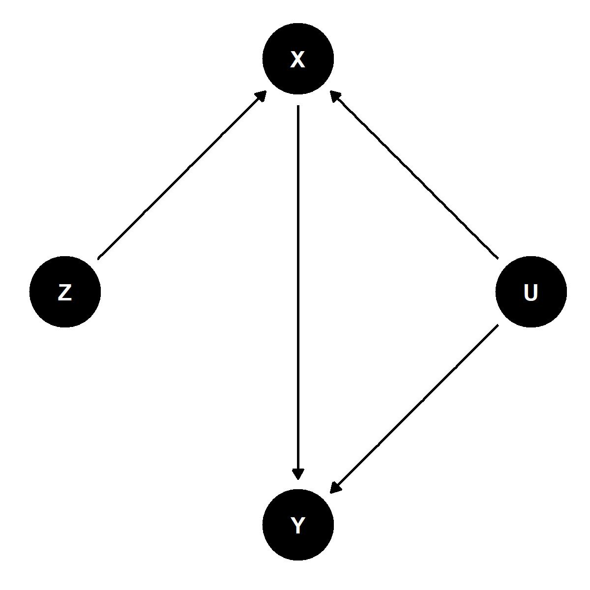
The above figure illustrates a causal relationship among four variables, only three of which we can observe and two of which we want to estimate the causal relationship between.
Y is our outcome of interest and X our explanatory variable. We would like to be able to identify the causal effect of X on Y. The problem, however, is that both X and Y are affected by some unobserved variable U. Unless we can account for U in our analysis our estimate of the effect of X on Y will not be accurate.
Enter our instrumental variable, Z. As the DAG above illustrates, while Y and X are both affected by U, only X is affected by Z and Z is independent of U. We can leverage this fact to our advantage. By isolating variation in X explained by Z we can identify the causal effect of X on Y. That’s pretty cool!
Now this approach comes with a necessary trade-off in generalizability. When we take an instrumental variables appraoch we’re estimating what’s called a local average treatment effect (LATE). This is in lieu of an average treatment effect (ATE). The “local” modifier alerts us to the fact that the effect of X on Y is identified by zeroing in on cases in our data that are best explained by the instrument Z. This loss of generalizability, while regrettable, comes with the reward that we can identify the causal relationship of interest.
A Simulation with seerrr
If the above is still too abstract, a simulation in R may help to make things more concrete (at least for R-users that are programmatically minded). Programming usually helps me grasp concepts that otherwise go over my head by letting me “tangibly” play with said concepts. Below, I do so using tools from the seerrr package.
First, I attach the seerrr package by writing:
library(seerrr)
Next, I prep some data for simulation. The data-generating process I’m going with is quite simple. For a sample of N = 1,000 observations I generate an “unobserved” normal variable U, an observed and exogenous instrument Z, my causal variable of interest X, and my outcome Y.
X is simply an additive function of the instrument Z, unobserved confounding U, and some random noise. Y conversely is an additive function of X, unobserved confounding, and some random noise.
By default simulate iterates the data-generating process 200 times. We’ll keep with that default and simulate the data as follows:
sim <- simulate(
  N = 1000,     # sample size
  U = rnorm(N), # unobserved confounder
  Z = rnorm(N), # observed instrument
  X = Z + U + rnorm(N), # causal variable
  Y = X + U + rnorm(N)  # outcome
)
By construction the true effect of X on Y is equal to 1 (Y = X + U = 1 \times X + 1 \times U, after all). In a world where we can observe U and control for it in a regression analysis, we can recover an unbiased estimate of the effect of X on Y quite easily.
We can check this using seerrr’s estimate function as follows and then using evaluate to evaluate the estimator’s performance:
# iteratively estimate linear model
cl_est <- estimate(
  data = sim, # simulated data
  Y ~ X + U,  # linear model specification
  "X",        # variable we're interested in
  se_type = "stata" # standard error type (HC1)
)
# evaluate its performance
evaluate(cl_est, truth = 1, what = "bias")
This gives us the following output:
# A tibble: 1 x 5
  term       bias      mse coverage power
  <fct>     <dbl>    <dbl>    <dbl> <dbl>
1 X     -0.000523 0.000499    0.947     1
When what = "bias" in evaluate the function returns for the variable of interest the average bias, mean squared error (mse), coverage of the 95 percent confidence intervals, and the power. The metric to pay closest attention to for our purposes is bias. Clearly, when we can directly control for U in our multiple regression model, the returned coefficient for X has very, very little bias.
So, here’s the problem… while we can observe U here (because this is a simulation), if we imagine a world where we can’t collect data on U we’re going to have a hard time getting an unbiased estimate of the effect of X on Y. Just look at what happens to the bias of our estimate when we don’t control for U:
lm_est <- estimate(
  data = sim, Y ~ X, "X", se_type = "stata"
)
evaluate(lm_est, truth = 1, what = "bias")
# A tibble: 1 x 5
  term   bias   mse coverage power
  <fct> <dbl> <dbl>    <dbl> <dbl>
1 X     0.334 0.112        0     1
Bias went way up. You may have noticed, too, that coverage is zero. That means our estimate for the effect of X on Y is so off base, the true effect isn’t even covered by the 95 percent confidence intervals in any of the iterations of the simulation. That’s pretty bad.
Thankfully, with the power of IV regression we can recover a more consistent estimate of X’s effect.
The workhorse IV approach used by researchers is two stage least squares (2SLS). This approach entails first regressing the causal variable of interest on an instrumental variable. Then, in the second stage, the response is regressed on the predicted values of the causal variable from the first stage regression.
To be consistent, the instrument needs to meet two criteria: (1) it needs to be relevant and (2) it needs to be exogenous. Instruments are said to be weak if they violate the first and estimates will be inconsistent if the second is violated. In the case of our simulation, we know the instrument Z meets both of these criteria (it does so by design). In real-world settings there are ways of verifying the validity of instruments. These methods are not perfect and require certain assumptions or conditions to hold. Nonetheless, it’s good to know what tools exist.
Getting back to our simulation, we can estimate and evaluate the performance of the IV approach quite easily. Using the iv_robust function from the estimatr package, we can easily compute the 2SLS estimate for the effect of X on Y as follows:
iv_est <- estimate(
  data = sim, Y ~ X | Z, "X", se_type = "stata",
  estimator = estimatr::iv_robust
)
Evaluating the results gives us the following:
evaluate(iv_est, truth = 1, what = "bias")
# A tibble: 1 x 5
  term       bias     mse coverage power
  <fct>     <dbl>   <dbl>    <dbl> <dbl>
1 X     -0.000304 0.00217    0.942     1
Bias is much improved! (And, notice that coverage is right back where it should be.) Because Z is a strong predictor of X and is exogenous, we can use it to localize variation in X that’s explained by Z to reliably identify X’s effect on Y. By doing this, all the variation in X that is explained by the confounding influence of U is eliminated. This leaves only the exogenous variation in X caused by Z for us to leverage to reliably estimate its effect on Y.
That’s IV and how to illustrate it with seerrr!