
Using R Markdown to Create Posts
I love working with R Markdown. It makes writing articles and putting together instructional materials easy, especially when they include statistical analysis or data visualizations. It turns out, I can use R Markdown to write blog posts, too.
I stumbled onto a helpful post by Steven Miller from 2019 that provides a nice summary of how to do this. I wanted to see how it worked myself, so I tried it out in writing this post.
To make it work I simply created a _source directory in the RStudio
project I use for my website. In that directory, I created and saved a
.Rmd file for this particular post. At the top of that file, I specified
the YAML as follows:
---
title: "Using R Markdown to Create Posts"
output:
  md_document:
    variant: gfm
    preserve_yaml: TRUE
knit: (function(inputFile, encoding) {
rmarkdown::render(inputFile, encoding = encoding, output_dir = "../_posts") })
author: "Miles D. Williams"
date: ""
excerpt: "Writing posts with R Markdown"
layout: post
categories:
  - R Markdown
  - Jekyll
---
The key to making this work is modifying the file path for knit.
Usually, when knitting a .Rmd file to an html or pdf the knitted version
is stored in the same working directory as the raw .Rmd file. I never
put together that one could customize where to store the knitted
version. For sites hosted by Jekyll (like mine), blog posts go in a
_posts directory. So, by specifying:
knit: (function(inputFile, encoding) {
  rmarkdown::render(inputFile, encoding = encoding, output_dir = "../_posts") })
I can keep the raw .Rmd file in one directory so that the only files
stored in the _posts directory are the actual blog posts I want to
publish on my site.
Then, all I need to do is knit the document and push the changes to GitHub. Voila, I have a blog post that also renders output from R code inline just as seamlessly as it would for any other document.
But, there is a caveat! I had to do two more things to make
everything work. First, I needed to set my working directory to the
_source directory where my .Rmd file lives. Next, I had to update my
setup code chunk to specify where to pull rendered figures from:
base_dir <- "~/My Website/milesdwilliams15.github.io/" # i.e. where the jekyll blog is on the hard drive.
base_url <- "/"
fig_path <- "assets/images/"

knitr::opts_knit$set(base.dir = base_dir, base.url = base_url)
knitr::opts_chunk$set(fig.path = fig_path,
                      cache.path = '../cache/',
                      message=FALSE, warning=FALSE,
                      cache = TRUE)
If the above isn’t specified, figures produced in R chunks won’t appear in the actual blog post because the knitted .md file will contain local file paths to the generated images by default—which is no good, no good at all.
Once all of that has been sorted out, making blogging with R Markdown work is as simple has pressing “Knit.” Everything should render just like it would in a knitted pdf or html. For instance, below is the boilerplate example text and R script you get when you open a .Rmd file in RStudio, with everything rendered just as it should be:
R Markdown
This is an R Markdown document. Markdown is a simple formatting syntax for authoring HTML, PDF, and MS Word documents. For more details on using R Markdown see http://rmarkdown.rstudio.com.
When you click the Knit button a document will be generated that includes both content as well as the output of any embedded R code chunks within the document. You can embed an R code chunk like this:
summary(cars)
##      speed           dist
##  Min.   : 4.0   Min.   :  2.00
##  1st Qu.:12.0   1st Qu.: 26.00
##  Median :15.0   Median : 36.00
##  Mean   :15.4   Mean   : 42.98
##  3rd Qu.:19.0   3rd Qu.: 56.00
##  Max.   :25.0   Max.   :120.00
Including Plots
You can also embed plots, for example:
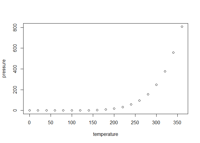
Note that the echo = FALSE parameter was added to the code chunk to
prevent printing of the R code that generated the plot.