When the Research Hypothesis Is the Null
What should you do if your research hypothesis is the null hypothesis? In other words, how should you approach hypothesis testing if your theory predicts no effect between two variables? I and a coauthor are working on a paper where a couple of our proposed hypotheses look like this, and we got some push-back from a reviewer about it. This prompted me to go down a rabbit hole of journal articles and message boards to see how others handle this situation. I quickly found that I waded into a contentious issue that’s connected to a bigger philosophical debate about the merits of hypothesis testing in general and whether the null hypothesis in particular as a bench-mark for hypothesis testing is even logically sound.
There’s too much to unpack with this debate for me to cover in a single blog post (and I’m sure I’d get some of the key points wrong anyway if I tried). The main issue I want to explore in this post is the practical problem of how to approach testing a null research hypothesis. From an applied perspective, this is a tricky problem that raises issues with how we calculate and interpret p-values. Thankfully, there is a sound solution for the null research hypothesis which I explore in greater detail below. It’s called a two one-sided test, and it’s easy to implement once you know what it is.
The usual approach
Most of the time when doing research, a scientist usually has a research hypothesis that goes something like X has a positive effect on Y. For example, a political scientist might propose that a get-out-the-vote (GOTV) campaign (X) will increase voter turnout (Y).
The typical approach for testing this claim might be to estimate a regression model with voter turnout as the outcome and the GOTV campaign as the explanatory variable of interest:
Y = α + β X + ε
If the parameter β > 0, this would support the hypothesis that GOTV campaigns improve voter turnout. To test this hypothesis, in practice the researcher would actually test a different hypothesis that we call the null hypothesis. This is the hypothesis that says there is no true effect of GOTV campaigns on voter turnout.
By proposing and testing the null, we now have a point of reference for calculating a measure of uncertainty—that is, the probability of observing an empirical effect of a certain magnitude or greater if the null hypothesis is true. This probability is called a p-value, and by convention if it is less than 0.05 we say that we can reject the null hypothesis.
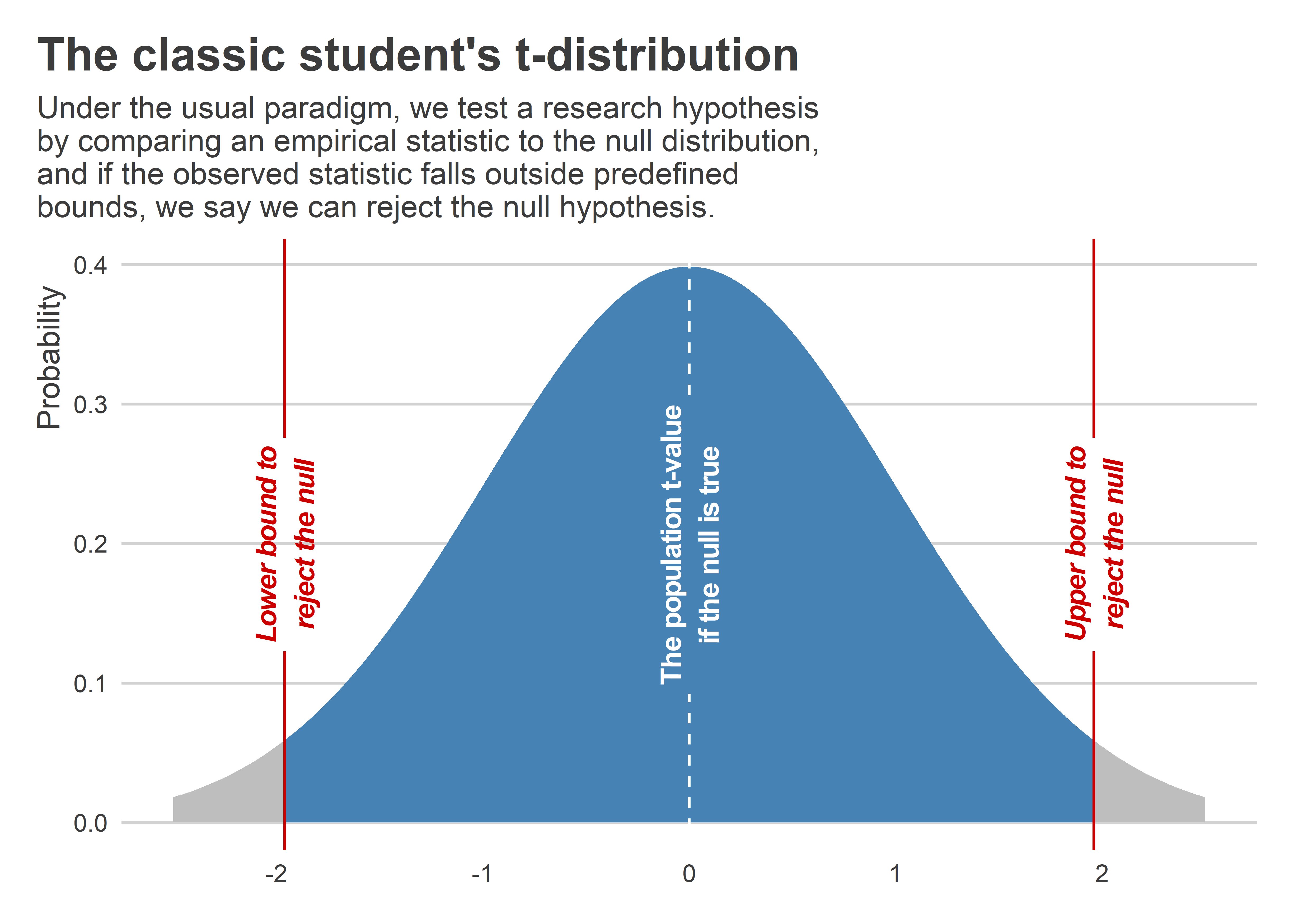
For the hypothetical regression model proposed above, to get this p-value we’d estimate β, then calculate its standard error, and then we’d take the ratio of the former to the latter giving us what’s called a t-statistic or t-value. Under the null hypothesis, the t-value has a known distribution which makes it really easy to map any t-value to a p-value. The below figure illustrates using a hypothetical data sample of size N = 200. You can see that the t-statistic’s distribution has a distinct bell shape centered around 0. You can also see the range of t-values in blue where if we observed them in our empirical data we’d fail to reject the null hypothesis at the p < 0.05 level. Values in gray are t-values that would lead us to reject the null hypothesis at this same level.

When the null is the research hypothesis we want to test
There’s nothing new or special here. If you have even a basic stats background (particularly with Frequentist statistics), the conventional approach to hypothesis testing is pretty ubiquitous. Things get more tricky when our research hypothesis is that there is no effect. Say for a certain set of theoretical reasons we think that GOTV campaigns are basically useless at increasing voter turnout. If this argument is true, then if we estimate the following regression model, we’d expect β = 0.
Y = α + β X + ε
The problem here is that our substantive research hypothesis is also the one that we want to try to find evidence against. We could just proceed like usual and just say that if we fail to reject the null this is evidence in support of our theory, but the problem with doing this is that failure to reject the null is not the same thing as finding support for the null hypothesis.
There are a few ideas in the literature for how we should approach this instead. Many of these approaches are Bayesian, but most of my research relies on Frequentist statistics, so these approaches were a no-go for me. However, there is one really simple approach that is consistent with the Frequentist paradigm: equivalence testing. The idea is simple. Propose some absolute effect size that is of minimal interest and then test whether an observed effect is different from it. This minimum effect is called the “smallest effect size of interest” (SESOI). I read about the approach in an article by Harms and Lakens (2018) in the Journal of Clinical and Translational Research.
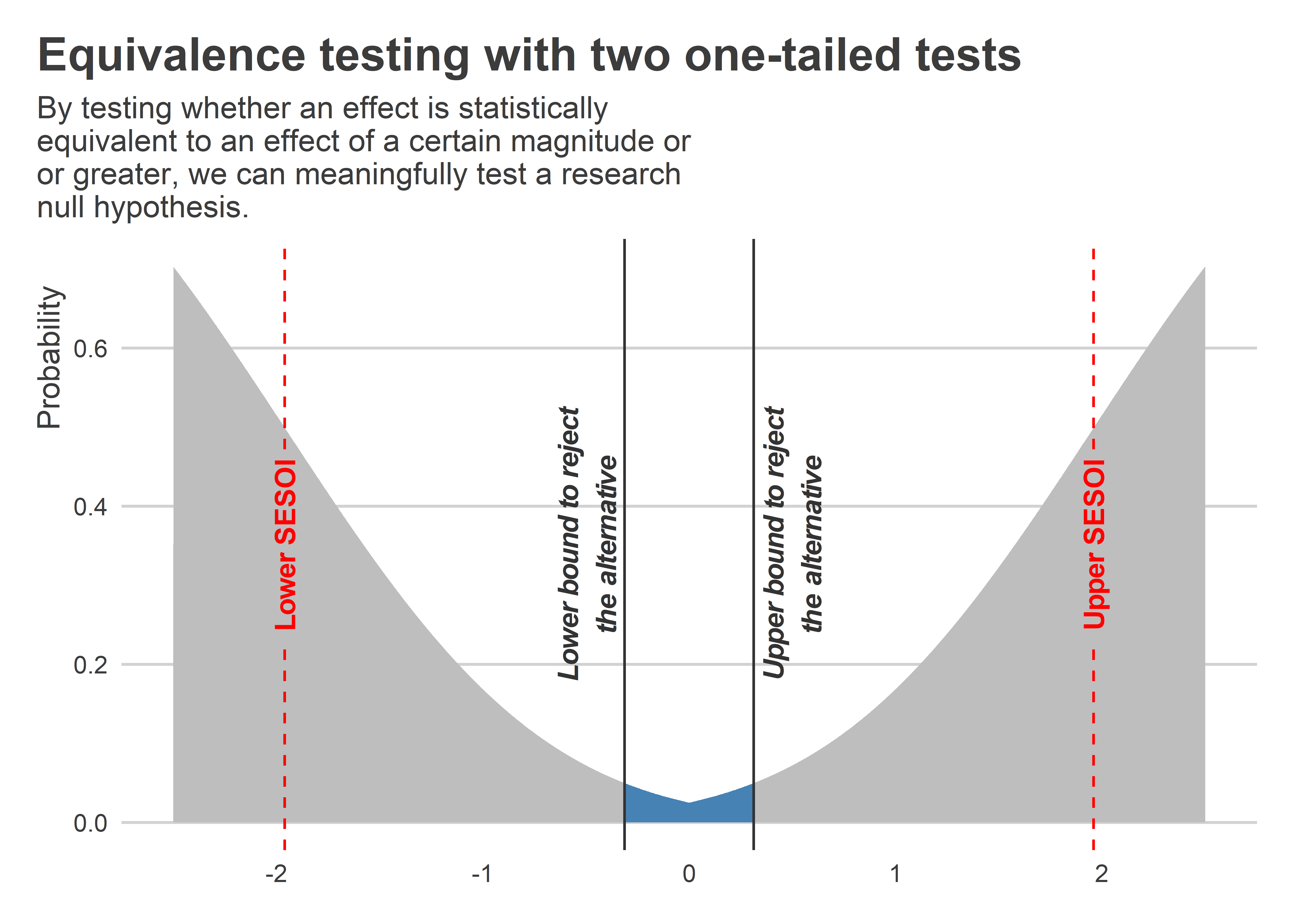
Say, for example, that we deemed a t-value of +/-1.96 (the usual threshold for rejecting the null hypothesis) as extreme enough to constitute good evidence of a non-zero effect. We could make the appropriate adjustments to our t-distribution to identify a new range of t-values that would allow us to reject the hypothesis that an effect is non-zero. This is illustrated in the below figure. We can now see a range of t-values in the middle where we’d have t-values such that we could reject the non-zero hypothesis at the p < 0.05 level. This distribution looks like it’s been inverted relative to the usual null distribution. The reason is that with this approach what we’re doing is conducting a pair of alternative one-tailed tests. We’re testing both the hypothesis that β / se(β) - 1.96 > 0 and β / se(β) + 1.96 < 0. In the Harms and Lakens paper cited above, they call this approach two one-sided tests or TOST (I’m guessing this is pronounced “toast”).

Something to pay attention to with this approach is that the observed
t-statistic needs to be very small in absolute magnitude for us to
reject the hypothesis of a non-zero effect. This means that the bar for
testing a null research hypothesis is actually quite high. This is
demonstrated using the following simulation in R. Using the {seerrr}
package, I had R generate 1,000 random draws (each of size 200) for a
pair of variables x and y where the former is a binary “treatment”
and the latter is a random normal “outcome.” By design, there is no true
causal relationship between these variables. Once I simulated the data,
I then generated a set of estimates of the effect of x on y for each
simulated dataset and collected the results in an object called
sim_ests. I then visualized two metrics that that I calculated with
the simulated results: (1) the rejection rate for the null hypothesis
test and (2) the rejection rate for the two one-sided equivalence tests.
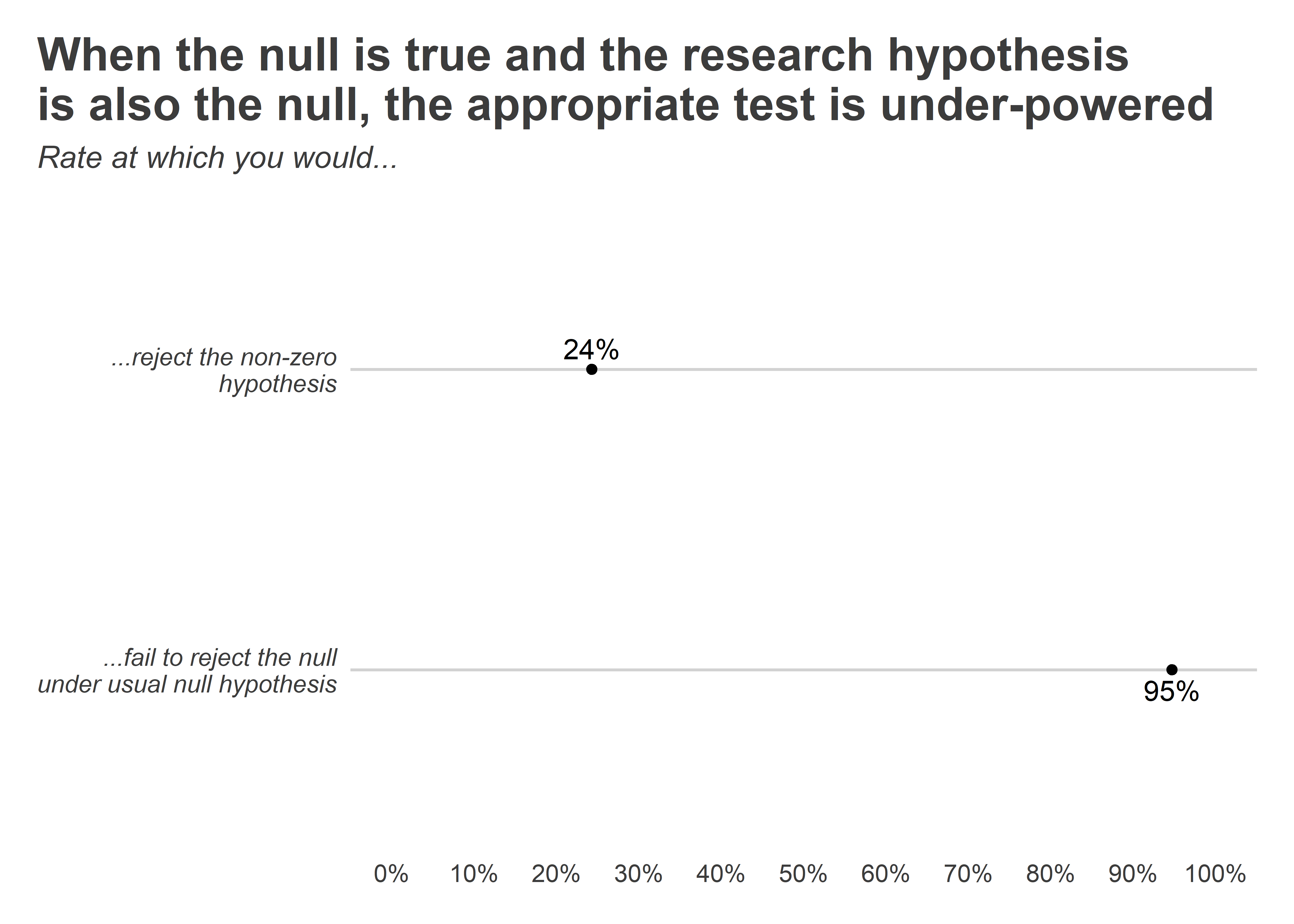
As you can see, if we were to try to test a research null hypothesis the
usual way, we’d expect to be able to fail to reject the null about 95%
of the time. Conversely, if we were to use the two one-sided equivalence
tests, we’d expect to reject the non-zero alternative hypothesis only
about 25% of the time. I tested out a few additional simulations to see
if a larger sample size would lead to improvements in power (not shown),
but no dice.
## open packages
library(tidyverse)
library(seerrr)

## run simulation and collect
## the results
simulate(
  R = 1000,
  N = 200,
  x = rbinom(N, 1, 0.5),
  y = rnorm(N)
) |>
  estimate(
    y ~ x,
    vars = "x",
    se_type = "stata"
  ) -> sim_ests

## make a function that returns
## the two one-side test p-value
alt_t <- function(
    tval, df, altval = 1.96
) {
  pt(abs(tval), df, altval)
}

## get this new p-value for each
## simulated estimate
sim_ests |>
  mutate(
    altpval = alt_t(statistic, df)
  ) -> sim_ests

## visualize the results
sim_ests |>
  summarize(
    nrt = mean(p.value <= 0.05),
    art = mean(altpval <= 0.05)
  ) |>
  ggplot() +
  geom_point(
    aes(
      y = "...fail to reject the null\nunder usual null hypothesis",
      x = 1 - nrt
    )
  ) +
  geom_point(
    aes(
      y = "...reject the non-zero\nhypothesis",
      x = art
    )
  ) +
  geom_text(
    aes(
      y = "...fail to reject the null\nunder usual null hypothesis",
      x = 1 - nrt,
      label = scales::percent(1 - nrt)
    ),
    vjust = 1.5
  ) +
  geom_text(
    aes(
      y = "...reject the non-zero\nhypothesis",
      x = art,
      label = scales::percent(art)
    ),
    vjust = -.5
  ) +
  labs(
    x = NULL,
    y = NULL,
    title = paste0(
      "When the null is true and the research hypothesis\n",
      "is also the null, the appropriate test is under-powered"
    ),
    subtitle = "Rate at which you would..."
  ) +
  scale_x_continuous(
    limits = 0:1,
    labels = scales::percent,
    n.breaks = 10
  ) +
  theme(
    panel.grid.major.x = element_blank(),
    plot.subtitle = element_text(face = "italic"),
    axis.text.y = element_text(face = "italic")
  )

Conclusion
The two one-sided tests approach strikes me as a nice method when dealing with a null research hypothesis. It’s actually pretty easy to implement, too. The one downside is that this test is under-powered. If the null is true, it will only reject the alternative 25% of the time (though you could select a different non-zero alternative which would possibly give you more power). However, this isn’t all bad. The flip side of the coin is that this is a really conservative test, so if you can reject the alternative that puts you on solid rhetorical footing to show the data really do seem consistent with the null.