A generalized correlation coefficient? Testing out ‘xi’

Back to Blog

Every now and again I stumble across an interesting new method. Usually these methods solve a highly technical or niche problem, but every now and again a new method is proposed that solves a very general and long-standing problem. The brand new coefficient of correlation created by Sourav Chatterjee falls into the latter category.

In a working paper simply titled “A New Correlation Coefficient”, Chatterjee describes an estimand called ξ that he claims solves the primary limitation of other correlation coefficients: their inability to detect non-linear, non-monotonic relationships between variables. In this post I want to explore this new ξ (pronounced “zee” and spelled “xi”) estimand and also consider whether it was really necessary.

TLDR: it’s a really cool method that I’ll keep in my toolbox, but it’s not really solving a problem that didn’t already have a (possibly better) solution.

The problem with most correlation coefficients

The correlation coefficient is ubiquitous in quantitative research. Nearly every intro course in statistical research methods talks about how to estimate correlations. The most commonly used is Pearson’s ρ (pronounced “row” and spelled “rho”) which quantifies how strong the linear correlation is between two factors and whether the direction of the relationship is positive or negative. If the value is 1, the relationship is perfectly linear and positive. If it’s -1, the relationship is perfectly linear and negative. If it’s 0, a linear relationship doesn’t exist.

Pearson’s ρ has a really simple formulation, and it has a direct correspondence to other foundational estimates of interest in statistics, like the mean and standard deviation, as well as linear regression. It also has this cool feature where if you square the estimated correlation coefficient, it gives you the share of the variation in the data explained by a linear relationship between the factors being studied.

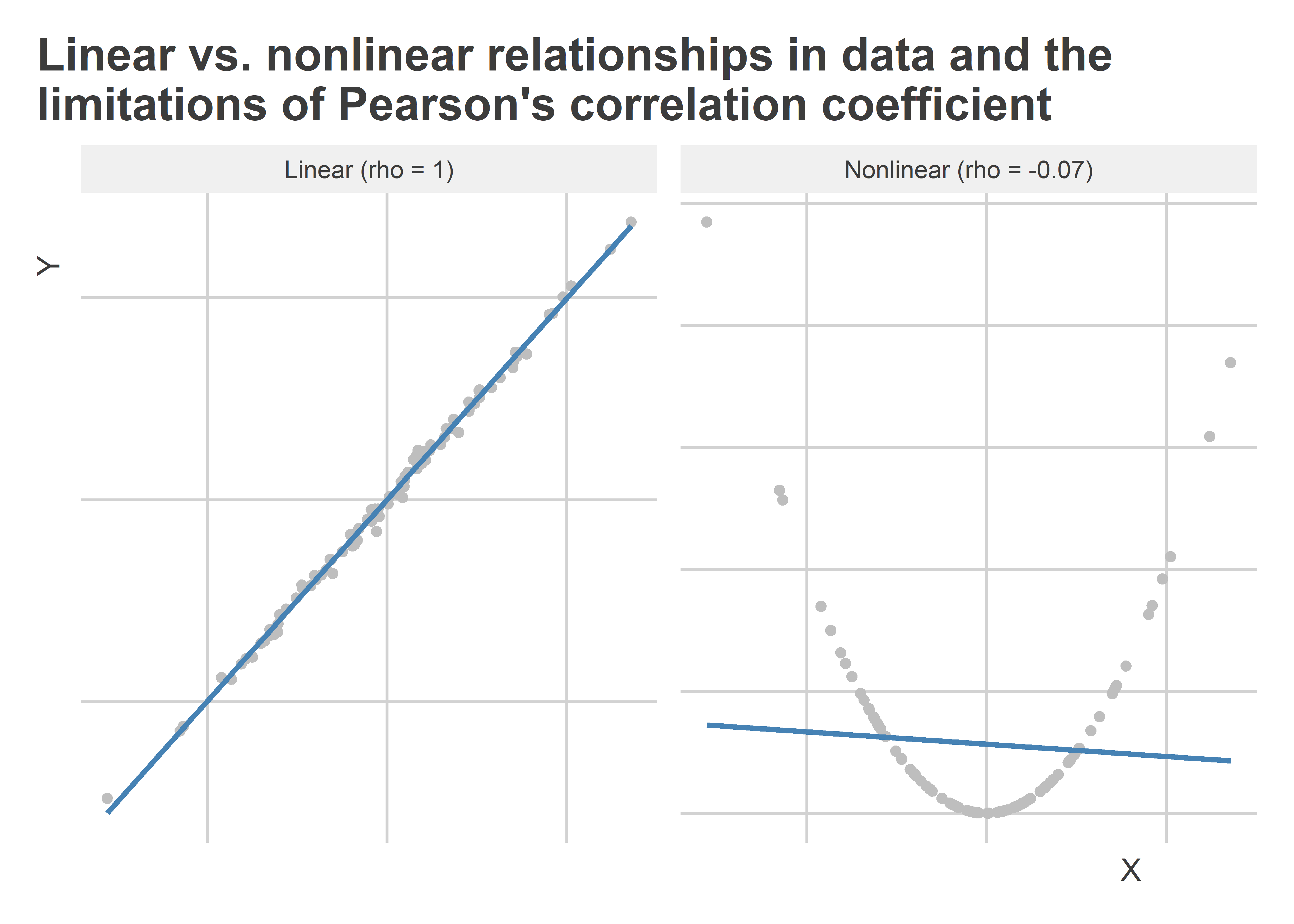
While simple to use, ρ’s main limitation is that if the relationship between two factors is non-linear, it’s going to be a bad metric of how strong their relationship is. Take the figure below, which shows two relationships between a variable “X” and a variable “Y” using scatter plots. Each includes a linear regression line and the estimated correlation coefficient. On the left, the underlying relationship is linear and very strong, and the estimate for ρ clearly reflects this (it’s 1 with some rounding). On the right, the underlying relationship is also very strong, but it is quadratic rather than linear. The estimate for ρ in this case is slightly negative and very close to zero. This is both accurate and misleading—accurate because the relationship isn’t linear (so ρ is doing its job) but misleading because there is a really strong relationship between X and Y.

This problem isn’t unique to Pearson’s ρ. To varying degrees, many other methods of quantifying the correlation between two factors have a similar limitation. So what are we supposed to do when we have data with a nonlinear relationship? Enter ξ.

A more general measure of correlation

The ξ correlation coefficient is supposed to be robust to nonlinear relationships in data. I’ll save the technical details for anyone who wants to read the paper. The gist of the idea behind ξ is that it provides a way of estimating whether two factors have a smooth relationship.¹ Whether that relationship is linear or not, doesn’t matter. If they do have a relationship, a 1 indicates the strongest possible correlation between factors, while a 0 indicates that the two factors are independent of each (not correlated).

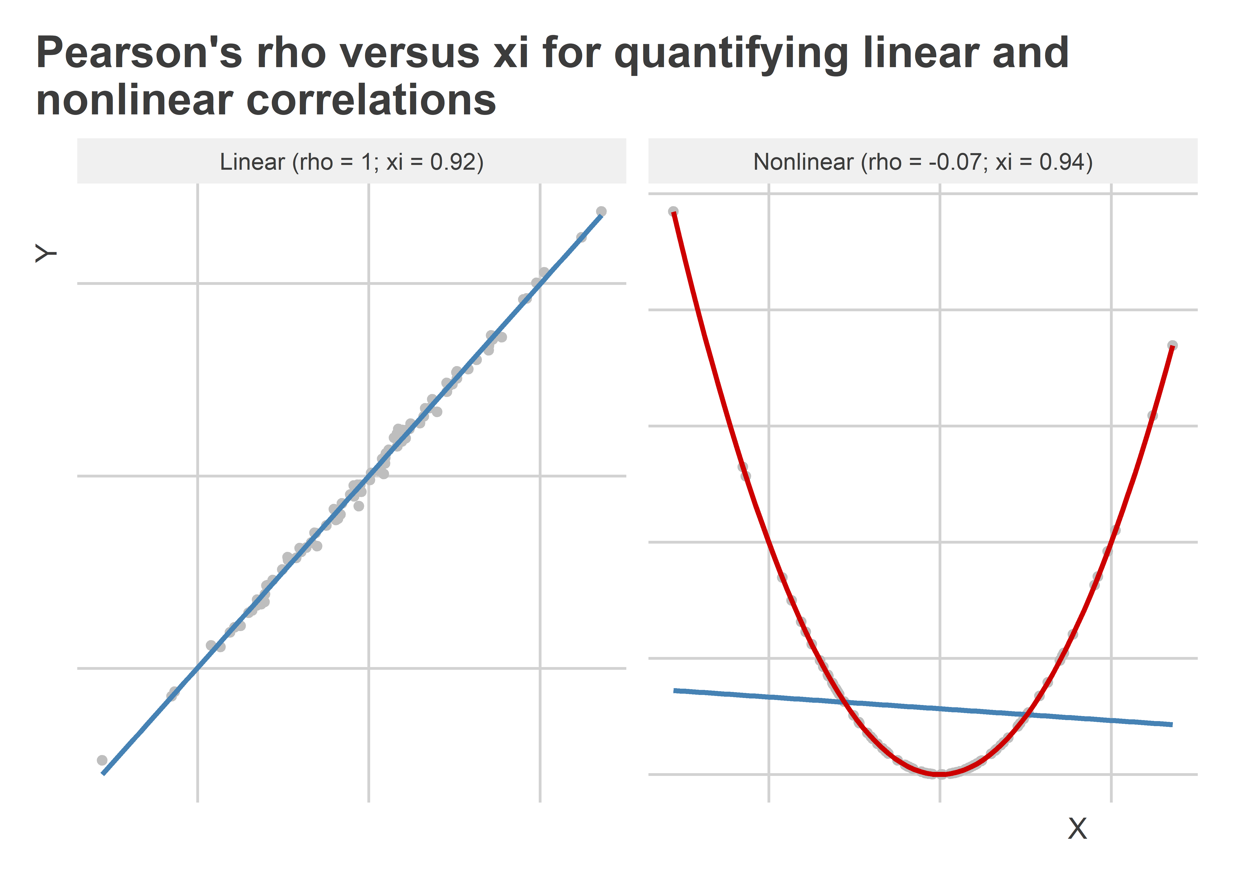
The next figure helps show what the ξ coefficient does for us. Using the same data as before, the estimate for ξ is shown alongside the estimate for ρ using both the linear and the nonlinear data. A red line is included in the nonlinear plot to summarize the nonlinear fit for the data provided by a more flexible generalized additive model (GAM) versus a linear model. We can see a few features of ξ immediately. First, it appears to be more conservative than ρ when the data are truly linear (ξ < ρ). In the paper by Chatterjee, he says this is the one major limitation of this correlation coefficient. By contrast, ξ redeems itself by its power to detect that the nonlinear data has a correlation that is equally as strong as that observed in the linear data. If anything, the estimate of ξ for the data on the right shows that the nonlinear relationship is stronger than the linear relationship in the data on the left. Go ξ!

Other means to the same end

When I first read the paper by Chatterjee, I was impressed. And while the math behind the method may seem dense to some, the formulation for ξ is actually pretty simple as far as novel statistical methods go. This impressed me, too.

There’s a lot going for ξ, but after giving it more thought, I realized that we already have some useful methods for detecting nonlinear relationships in data and quantifying their strength. One simple idea I had is to simply use the R-squared from a generalized additive model or GAM like the one fit to the nonlinear data in the last section. The below figure shows the estimate we get using this approach with both the linear and nonlinear data alongside ρ and ξ. Because we’re already using Greek letters, let’s call the GAM estimate of the correlation γ (“gamma”—see what I did there?). This approach works by fitting two GAMs to the data where the two variables of interest are used alternately as the right-hand-side and left-hand-side variables in a GAM regression. The R-squared is then calculated for each fit and the greater of these two values is reported. As you can see in the figure below, this approach is just as powerful as ρ in detecting a linear relationship and even more powerful than ξ in detecting a strong nonlinear relationship.

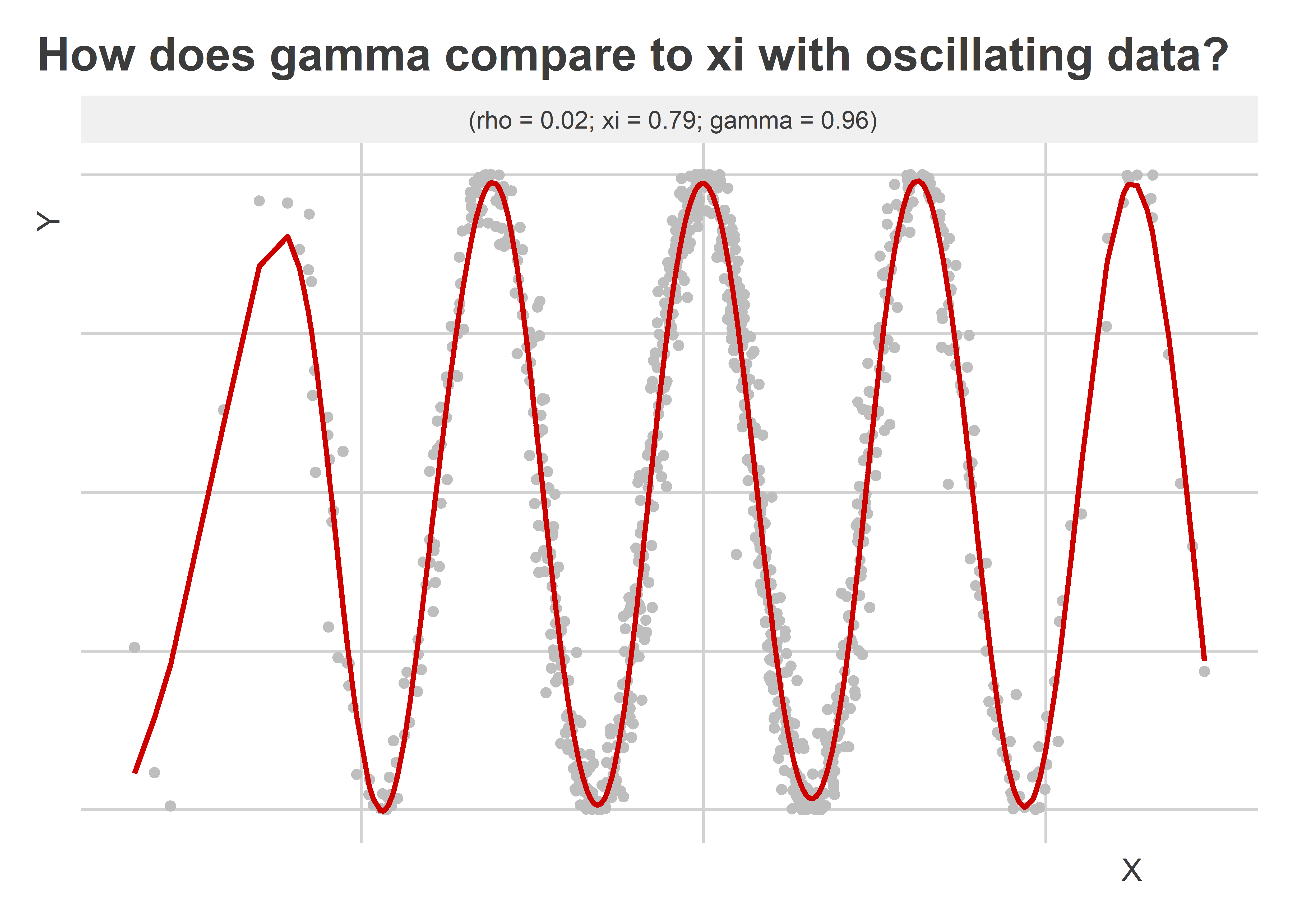
An even tougher test of this approach relative to ξ would be to have some data where we observe oscillations. The below figure shows what happens with this kind of data. I generated a variable “X” that consists of random draws from a normal distribution and a variable “Y” which is just the cosine of X (plus a little extra noise). I plotted the data in scatter plot and fit a GAM regression line to the data with the appropriate settings for picking up a smooth but oscillating pattern in the data. Comparing the estimates of ρ, ξ, and γ, we can see that only the latter two are capable of detecting that a relationship exists between X and Y. While both indicate that the relationship is strong, γ is slightly better powered.

Ultimate takeaways

I like ξ a lot, and if you want to use it, Chatterjee created an R package called {XICOR} that you can install directly from the CRAN. It’s just as easy to use as cor() in base R, and it also reports either asymptotic or Monte Carlo based p-values. All of these are major pros for this method.

I don’t think ξ is solving a problem that didn’t already have a solution, though. The γ coefficient I came up with appears to be better powered than ξ with nonlinear data.

Also, another benefit of γ that I didn’t mention above is interpretation. While I get that ξ can take a value from 0 to 1 where 1 means the strongest possible correlation and 0 means no correlation, I don’t quite know what ξ means in substantive terms. It doesn’t seem to be a summary of the variation explained in the data from the correlation between two factors. By comparison, γ does have this kind of substantive interpretation.

So which estimand should you choose? I don’t see this as an either-or question. I will definitely keep ξ in my toolbox. It just won’t be replacing any other tools that I already have.

For anyone interested

For anyone interested, here’s some R code for estimating γ (“gamma”).

library(mgcv)
gammacor <- function(x, y, k = 5) {
  ## shortcut to only keeping pairwise valid values
  mf <- model.frame(y ~ x)
  
  ## GAM with y ~ x
  gam(
    y ~ s(x, k = k), data = mf
  ) -> fity
  
  ## GAM with x ~ y
  gam(
    x ~ s(y, k = k), data = mf
  ) -> fitx
  
  ## return max r-squared
  pmax(
    cor(fitted(fity), mf$y)^2,
    cor(fitted(fitx), mf$x)^2
  )
}

## example
x <- rnorm(1000, sd = 5)
y <- cos(x + rnorm(1000, sd = 0.2))
gammacor(x = x, y = y, k = 25)

## [1] 0.9643008