
Stop telling people to produce a histogram of regression model residuals
Andrew Gelman and Jennifer Hill write in their classic book, Data Analysis Using Regression and Multilevel/Hierarchical Models, one of the least important assumptions of a linear regression model are the equal variance (homoskedasticity) and normality of errors. In fact, in their book, they explicitly advise against checking for normality by producing a histogram of the model residuals, and they advise against checking for equal variance by producing a scatter plot of the model residuals against the model fit. This was the same advice I received in grad school in my statistical methods training.
Not everyone seems to have received this advice, even some very smart and otherwise well trained quantitative social scientists and some folks in the harder sciences like biology or physics. This is bad for two reasons, the first of which is that it’s bad statistical practice. The second reason it’s bad is that the folks who adopt this practice teach it to others.
So, why is it bad? So many online sources talk about the importance of equal variance and normality of errors in regression analysis. In this post, I’ll run a few simple simulations that show why these assumptions just aren’t that important or even worth checking.
The assumptions that matter
Andrew Gelman summarized the key assumptions of the linear regression model in a blog post that amazingly is more than 10 years old now. The two most important assumptions are as follows:
- Validity. Most importantly, the data you are analyzing should map to the research question you are trying to answer. This sounds obvious but is often overlooked or ignored because it can be inconvenient…
- Additivity and linearity. The most important mathematical assumption of the regression model is that its deterministic component is a linear function of the separate predictors…
In short, you should have good data and the best model of the outcome you wish to study should be additive and linear. That’s it. If you want to make causal claims, you need to assume a few more things, but in no instance does checking the above assumptions or those additional assumptions for causal inference require looking at model residuals.
The assumptions that matter less
The three additional assumptions of linear regression are:
- Independence of errors. . . .
- Equal variance of errors. . . .
- Normality of errors. . . .
Some people add the assumption that the error term is mean-zero as well, though in reality this is more a property of using OLS to estimate the regression model than an assumption that can be verified.
The important thing to remember with the above three is that they are of lower-order importance because they have only a very small bearing on model fit. Where these assumptions become more important is in making statistical inferences. To put it a little more formally, if we have a linear regression model of the form:
\[y_i = \beta_0 + \beta_1x_i + \epsilon_i\]the above assumptions are not necessary for obtaining an unbiased estimate of the slope (\(\beta_1\)) and intercept (\(\beta_0\)). As long as we have good data and a linear additive functional form is the best model for the outcome, using OLS to estimate the model will give us a good fit for the expected value or conditional mean of \(y_i\). Of course, if we cared about getting observation-specific predictions, this would be a different story, but this rarely is a concern in most quantitative scientific research.
Independence, equal variance, and normality of the error term are important if we care about making good statistical inferences. That is, if we want to have unbiased estimates of \(\text{var}(\beta_1)\) and \(\text{var}(\beta_0)\), then we should care about these assumptions.
Thankfully, we don’t have to change anything about the way we estimate the regression model to correct for violations of these assumptions. We can just use robust standard errors to deal with violations of equal variance and normality and include clustering to deal with a violation of independence.
Now, I know what you’re thinking. Wouldn’t we want to check the residuals to see if we need to use robust standard errors or clustering? The answer, again, is NO. The reason is that (1) robust standard errors provide the appropriate coverage whether or not equal variance and normality are violated, so you can just use them; and (2) there can be violations of these assumptions of unknown form that will not be obvious to the naked eye.
In short, checking the residuals is unnecessary and potentially misleading because violations of assumptions will not always be obvious. So, don’t do it.
A simulation
To quickly show that violations of 3-5 don’t matter for model fit (e.g., bias), let’s run a simple simulation. The below code simulates multiple draws from four data-generating processes for an outcome \(y_i\):
-
\(y_i = x_i + \epsilon_i\); \(\epsilon_i \sim \mathcal{N}(0, 1)\)
-
\(y_i = x_i + \mu_i + \epsilon_i\); \(\epsilon_i \sim \mathcal{N}(0, 1)\) and \(\mu_i \sim [\mathcal{N}(0, 1)]^2\)
-
\(y_i = x_i + \gamma_k + \epsilon_i\); \(\epsilon_i \sim \mathcal{N}(0, 1)\) and \(\gamma_k \sim [\mathcal{N}(0, 1)]\) for \(K = 10\) clusters.
-
\(y_i = x_i + \gamma_k + \mu_i + \epsilon_i\); \(\epsilon_i \sim \mathcal{N}(0, 1)\), \(\mu_i \sim [\mathcal{N}(0, 1)]^2\), and \(\gamma_k \sim [\mathcal{N}(0, 1)]\) for \(K = 10\) clusters.
In (1), the error term is independently distributed, has equal variance, and is normally distributed. In (2) non-normality (and thus also unequal variance) is introduced in the form of a squared stochastic term. In (3) non-independence is introduced in the form of a cluster-specific stochastic term. In (4), a combination of (2) and (3) is introduced.
## open the packages I need:
library(tidyverse)
library(seerrr)
library(coolorrr)
set_theme()
set_palette()

## draw multiple datasets from the possible dgps:
simulate(
  ## no. of iterations and sample size
  R = 1000,
  N = 500,

  ## the explanatory variable and unobserved errors
  x = rnorm(N), # the predictor
  e = rnorm(N), # the iid error term
  u = rnorm(N)^2, # the non-normal error term
  v = sample(rnorm(10), N, T), # the clustered error term

  ## the models:
  ## independence, equal variance, and normality are met
  y1 = x + e,

  ## normality and equal variance is violated
  y2 = x + u + e,

  ## independence is violated
  y3 = x + v + e,

  ## all the assumptions are violated
  y4 = x + u + v + e
) -> sim_dt
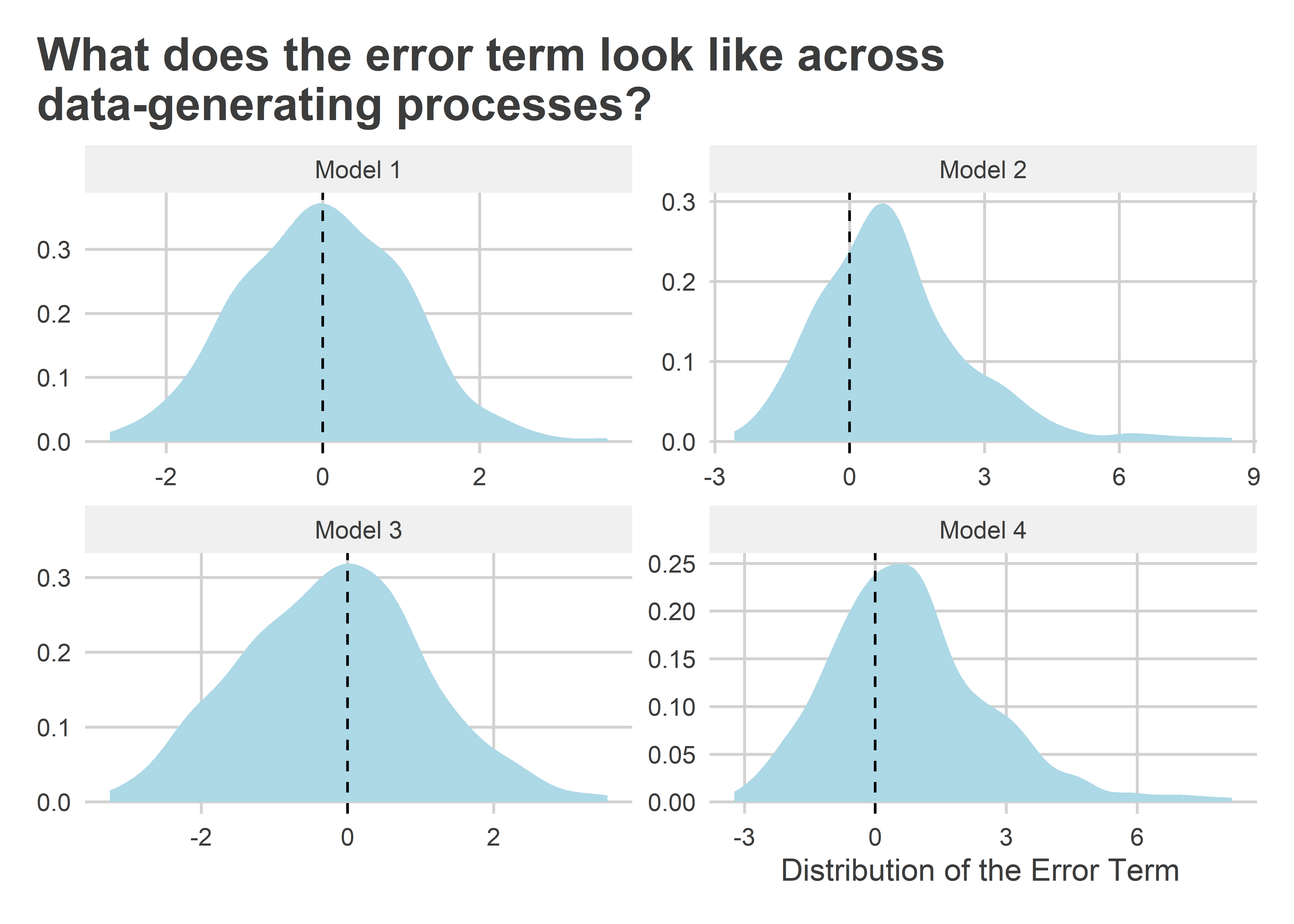
To show that the errors for data-generating processes 2-4 are not normal, here are some histograms of what the stochastic component of each model looks like for one of the datasets simulated above. We can clearly see violations of normality in (2) and (4), but clustering is not quite so obvious in (3); though it is clear that the distribution is a little fatter than the standard normal distribution.
sim_dt[[1]] |>
  transmute(
    "Model 1" = e,
    "Model 2" = e + u,
    "Model 3" = e + v,
    "Model 4" = e + u + v
  ) |>
  pivot_longer(everything()) |>
  ggplot() +
  aes(x = value) +
  facet_wrap(~ name, scales = "free") +
  geom_density(
    fill = "lightblue",
    color = "lightblue"
  ) +
  geom_vline(
    xintercept = 0,
    linetype = 2
  ) +
  labs(
    x = "Distribution of the Error Term",
    y = NULL,
    title = "What does the error term look like across\ndata-generating processes?"
  )
How problematic are these violations of linear model assumptions? Let’s estimate the model parameters for each of the simulated datasets to see:
list( ## list of the different model formulas
  y1 = y1 ~ x,
  y2 = y2 ~ x,
  y3 = y3 ~ x,
  y4 = y4 ~ x
) |>
  map_dfr( ## generate distribution of estimates for each model
    ~ estimate(
      data = sim_dt,
      formula = .x,
      vars = "x",
      se_type = "stata",
      clusters = ifelse( ## make sure to cluster ses for (3) and (4)
        names(.x) %in% c("y3", "y4"),
        as.factor(v),
        NULL
      )
    )
  ) -> sim_est
With the distribution of estimates collected, it’s time to evaluate the results and collect the summary:
sim_est |>
  group_split(outcome) |>
  map_dfr(
    ~ evaluate(
      data = .x,
      what = "bias",
      truth = 1
    ) |>
      mutate(
        outcome = unique(.x$outcome)
      )
  ) -> sim_evl
Now, we just need a simple visualization to report the output. The below figure shows the average of the model estimates along with the 95% confidence interval for the distribution of estimates. The coverage provided by the robust standard errors is indicated as well. For a test to reject the null at the standard \(p < 0.05\) level, we should expect the coverage to be 95%. The results below show (1) negligible bias in model estimates, (2) that non-normal and non-independent errors increase the estimated variance of model estimates, and (3) despite the increase in variance the standard errors still have the appropriate coverage for a test to reliably reject the null with the correct false positive rate at the standard threshold of \(p < 0.05\).
ggplot(sim_evl) +
  aes(
    x = average,
    y = reorder(outcome, 4:1),
    xmin = average - 1.96 * sqrt(variance),
    xmax = average + 1.96 * sqrt(variance)
  ) +
  geom_pointrange(
    color = "navy"
  ) +
  geom_label(
    aes(x = 0.95,
        label = paste0(round(coverage * 100, 2),"% Coverage")),
    color = "gray40",
    vjust = -0.6
  ) +
  geom_vline(
    xintercept = 1,
    linetype = 2
  ) +
  labs(
    x = "Average Point Estimate with 95% CIs",
    y = NULL,
    title = "How do non-iid errors affect OLS estimates?"
  )

The bottom line
Violations of normality and equal variance of the error terms are not the most important things to consider when studying data with linear regression models. Especially if the goal is to obtain an unbiased estimate of the conditional mean of an outcome given some variables, violations of these kind matter very little. Even if independence is violated, this is no major concern. Where these kinds of issues do warrant attention is statistical inference, but thankfully we have variance estimators that are robust to deviations from the classical assumptions of linear regression.
The most important assumptions for using linear regression are:
- That you have good data.
- That an additive, linear model is the best model for the data.
You need some additional assumptions if you want to use linear regression to estimate causal effects, but I’ve discussed some of those assumptions in other posts. Whatever the case, you certainly don’t need to make histograms of model residuals or create plots of model residuals by model fit to diagnose violations of assumptions about the error term. So don’t do it!