
Bear Braumoeller and Systemic Theory
The untimely passing of Dr. Bear Braumoeller still fills me with disbelief. As the many kind words of individuals on Twitter attest, the OSU professor was not only a giant in the field of security studies but also a kind and supportive colleague and friend to many.
On only one occasion did I have a chance to meet Bear in person. When I was a grad student at UIUC, I gave Bear a ride to the political science department from his hotel back in fall of 2019 during a visit. He was there to talk about his latest book, an important and accessible read making a data-driven argument about the persistence of international war in the modern era. It was a powerful rebuttal to some claims made by other prominent scholars espousing the so-called “decline of war thesis,” which holds that war is going out of fashion. Bear’s book relies on a distinct mix of advanced statics and diplomatic history to convince you otherwise.
I quickly devoured the book before Bear arrived at UIUC and hoped to talk with him about it. Unfortunately, as a star-struck third-year Ph.D. student at the time, I choked during the car ride and could muster little more than small talk.
It’s hard meeting your heroes, and Bear was one of mine. His first book, The Great Powers and the International System, is just as timeless a read as his second book. When I first read it as a master student back in 2016, it solidified my interest in studying International Relations. I knew then that I wanted to make a career out of studying big questions in international politics. Bear would never know it, but he’s one of the reasons I knew I wanted to get a Ph.D. in political science and pursue an academic career.
Years later, I’m (thankfully!) an employed academic at Denison University. And even more, given its location just outside Columbus, OH, I now live within only a few square miles of Bear’s stomping grounds. After using his second book for one of the classes I taught in the Fall of 2022, I decided to reach out to him via email. I told him not only that I had a fun time using the book in class, but that I also created a web application based on the data he used in the book so my students could explore the data. I also took the opportunity to solicit some of his feedback on a research note his book inspired me to write dealing with the some of the technical details of statistically measuring trends in the intensity of war.
Bear’s response was generous. He expressed excitement about the app I created and provided me with helpful feedback on my research note, offering to take a second look if I chose to continue with project. Since he was in Oslo working on research of his own, I didn’t have a chance to meet with him in person in Columbus, but hoped I might be able to touch base with him when he returned.
Sadly, this was not to be as Bear passed away in May of 2023. If my short correspondence with Bear was enough to make his passing a shock, the effect on the broader community of scholars in his network was exponentially greater—not to mention his family.
I’m in no position to offer a eulogy. I’m far too new and peripheral a member of Bear’s network. Instead, in my own weird way, I want to honor his memory by writing a post on how to program Bear’s model of systemic politics. This model forms the foundation of his first book as well as an article he published a few years prior in APSR.
As my friend Ekrim Baser tweeted after Bear’s passing, Bear’s systemic approach wasn’t given the attention it deserved. “IR desperately needs more general equilibrium thinking. We should be rewarding the precious few people who are crazy enough to push us in that direction,” Ekrim further noted.
Now, let’s get real for a second. You have to be a little crazy to engage in general equilibrium thinking. It can be mind-bendingly hard. However, the payoffs are exponential once you get past the initial trepidation and upstart costs.
In this post, I want to do my best to pay some of these upstart costs up front. As inaccessible Bear’s systemic theory was to me upon my first reading, it became far clearer when I started to get my hands dirty with it. By “getting my hands dirty,” I mean programming. As with most advanced concepts, I personally find that I don’t truly understand them until I can program them. That’s just what I did with Bear’s model of systemic politics, and detailing how I did this is what I’d like to do with the remainder of this post.
So, without further ado…
What is Systemic Politics?
Braumoeller’s model of systemic politics was his answer to the “agent-structure problem” in international relations. Do agents act upon their environment, or does their environment determine their behavior? The answer of course is that agents both shape, and are shaped by, the structures around them. Recognition of this fundamental truth is what makes Braumoeller’s theory truly systemic, namely, that it characterizes the dynamic feedback loop between structure and agents.
Because it reflects “big picture” thinking, the theory’s predictions are not so fine-grained as to be able to forecast the foreign policy activities of states or the occurrence and outcomes of wars. Rather, the theory offers predictions about how active states will be in international politics (from isolationist to highly internationalist) and how their activities will shape the distribution of different things states care about, like power or the spread of ideology.
This is not to say that systemic politics offers nothing of value to questions about the specific foreign policy choices of countries. It can be combined with lower-level theories to explain the specific forms that a country’s activity might take, as Braumoeller does in other work examining militarized interstate disputes. Nonetheless, the generic framework is not tooled specifically to deal with the day-to-day choices of leaders or the outcomes of those choices. It is more sweeping than that, dealing instead with the process by which the international system comes to settle into a general equilibrium between the activity levels of states and the structures they inhabit.
The Mathematical Model
Braumoeller captured the interplay of agents and structure in the form of a mathematical model that describes the activities of agents and the structures around them. Rather than game theoretic, the model is descriptive, which is not the same as saying it is devoid of theory or mechanisms.
The model itself is comprised of a system of differential equations relating the activities of an arbitrary number of countries to the state of the world along an arbitrary number of dimensions in the international system. For a country c ∈ 1, …, c, …, N, its level of activity ac ≥ 0 at time t + 1 is given as:
ac(t+1) = Σdωd[vc(cd)−sd(t)]2
In the above, state c’s activity level at a point in time is a function of its level of dissatisfaction between the state of the system (sd) along each dimension d ∈ 1, …, d, …, M (these might be the distribution of power, ideology, etc.) at time t and its ideal point for a given dimension (vc(cd)). The value cd is a frequency distribution of the attitudes of individuals within a country with respect to a given dimension of the international structure, and vc(⋅) is a preference aggregation function that maps the attitudes of individuals to a country-level preference about the the state of the system in dimension d. The weight placed on a given dimension is determined by the state’s worldview ωd ≥ 0 (i.e., how much the country cares about power or the spread of its preferred ideology).
We can see from the above that the extent to which a country is internationalist versus isolationist is proportional to (1) the difference between the state of the world and a country’s ideal state of the world and (2) the weight a country attaches to different dimensions of the state of the world.
The change produced by the collective activities of N countries in dimension d is then defined as:
Δ sd(t) = Σcπcωdac(t)[vc(cd)−sd(t)]
Or, if you like:
sd(t+1) = Σcπcωdac(t)[vc(cd)−sd(t)] + sd(t)
In the above, the difference between a country’s ideal point and the state of the system determines the direction that a country’s activity pushes the state of the system along a given dimension. The relative force behind this push is determined by the country’s overall dissatisfaction with the state of the world, how internationalist it is (its level of activity), the strength of the country’s worldview, and a new factor (πc) which denotes the state’s relative realized capabilities scaled to 0 ≤ πc ≤ 1.
These equations, depending on the starting values of the model’s exogenous parameters, allow for a dynamic feedback loop between the state of the system and the level of activity of countries until the system eventually settles into an equilibrium where activity levels and the state of the world remain constant.
Programming and Simulating the International System
This mathematical model lends itself well to simulation. It can create
some headaches when it comes to programming it, however. So I’ll walk
through my approach slowly, explaining the code along the way (though
you at minimum will need to be familiar with R for any of this to make
much sense). I’ve done the programming in R, restricting myself to
{baseR} as much as possible, saving the {tidyverse} for
visualization.
First, we need to create a function for activity given country world
views, ideal points, and the current state of the system. The below
function will accept a matrix w, a matrix v, and a vector s that
provide the relevant information. This function is generalized to any
arbitrary number of structural dimensions and countries. For w and
v, information in columns will be for each country in the
international system, and rows will denote dimensions for the state of
the world. s will just be a vector denoting the starting values for
the state of the system for each of M arbitrary dimensions.
## Create function for agent activity:
activity <- function(w,v,s){
  a <- 0
  for(i in 1:ncol(w)) {
    a[[i]] <- sum(w[, i] * (v[, i] - s)^2)
  }
  a
}
Say we have the following values for a pair of countries and one dimension characterizing the state of the world. If we test our activity function with the below inputs, we should see that country A is isolationist while B is internationalist. The reason is that, in the below code, the state of the world along the one dimension of relevance to our countries is equal to A’s ideal point, but not B’s.
w <- cbind(c(0.5), c(0.5))
v <- cbind(c(0.5), c(1))
s <- 0.5
activity(w, v, s)
## [1] 0.000 0.125
Next, we need a function that tells us how the structure of the system
changes given the activity of countries. The below function takes the
same inputs as before (w, v, and s) and adds a vector a for
country activity levels and a vector p for a county’s relative
realized capabilities.
## Create function for structure:
structure <- function(a,p,w,v,s){
  d.s <- 0
  for(d in 1:length(s)) {
    d.s[d] <- sum(p * w[d, ] * a * (v[d, ] - s[d]))
  }
  d.s + s
}
If we run this function using the output from the activity function and the other values specified above with the added specification of relative capabilities, the function returns a new state of the world for time t + 1.
p <- c(0.5, 0.5)
a <- activity(w, v, s)
structure(a, p, w, v, s)
## [1] 0.515625
Finally, we need a function that will let activity and structure play out over time. The below function lets the system run for a default of 20 time periods. It returns a list of objects: a data frame of country activity levels over time and a data frame of the state of the system over time, respectively.
## Create function to let the system evolve
system <- function(p,w,v,s,periods=20){
  s.start <- s
  a.out <- list()
  s.out <- list()
  for(t in 1:periods) {
    a <- activity(w=w,v=v,s=s)
    s <- structure(a=a,p=p,w=w,v=v,s=s)
    a.out[[t]] <- data.frame(
      a = a,
      t = t,
      state = LETTERS[1:ncol(w)]
    )
    s.out[[t]] <- data.frame(
      s = s,
      t = t+1,
      dimension = as.factor(1:length(s))
    )
  }
  s.out.start <- data.frame(
    s = s.start,
    t = 1,
    dimension = as.factor(1:length(s))
  )
  s.out <- rbind(
    s.out.start,
    do.call(rbind,s.out)
  )
  list(
    activity = do.call(rbind,a.out),
    structure = s.out
  )
}
Given the above values, we can check what this looks like:
system(p, w, v, s, periods = 5)
## $activity
##               a t state
## 1  0.0000000000 1     A
## 2  0.1250000000 1     B
## 3  0.0001220703 2     A
## 4  0.1173095703 2     B
## 5  0.0004449138 3     A
## 6  0.1105299244 3     B
## 7  0.0009167173 4     A
## 8  0.1045074047 4     B
## 9  0.0014989741 5     A
## 10 0.0991222132 5     B
##
## $structure
##           s t dimension
## 1 0.5000000 1         1
## 2 0.5156250 2         1
## 3 0.5298300 3         1
## 4 0.5428186 4         1
## 5 0.5547535 5         1
## 6 0.5657665 6         1
Finally, to make plotting more convenient, the below function will take
the output from system() and show how activity and the state of the
system change over time. (Here’s the bit where I deviate from only using
{baseR}.)
## Create a function to plot how the system changes
library(tidyverse)
library(patchwork)
sys_plot <- function(sys.out,
                    xlab='time',
                    ylab=c('activity','structure'),
                    str.names,
                    act.names) {
  p1 <- sys.out$activity %>%
    ggplot() +
    aes(
      t,a,linetype=state
    ) +
    geom_line() +
    labs(
      x = xlab,
      y = ylab[1],
      linetype = "Country"
    ) +
    scale_x_continuous(
      breaks = NULL
    ) +
    scale_y_continuous(
      breaks = NULL
    ) +
    theme_classic() +
    theme(
      legend.position = 'top',
      legend.title = element_text(face=4)
    )
  p2 <- sys.out$structure %>%
    ggplot() +
    aes(
      t,s,linetype=dimension
    ) +
    geom_line() +
    scale_x_continuous(
      breaks = NULL
    ) +
    scale_y_continuous(
      breaks = NULL
    ) +
    labs(
      x = xlab,
      y = ylab[2],
      linetype = "Balance of..."
    ) +
    theme_classic() +
    theme(
      legend.position = "top",
      legend.title = element_text(face=4),
      axis.text.y = element_text(angle = 90, hjust = .5)
    )
  if(!missing(act.names)) p1 +
    scale_linetype(
      breaks = unique(sys.out$activity$state),
      labels = act.names
    ) -> p1
  if(!missing(str.names)) p2 +
    scale_linetype(
      breaks = unique(sys.out$structure$dimension),
      labels = str.names
    ) -> p2
  p1 + p2
}
Let’s take the above example, and show how it plays out. Note how little code I need to write (now that I’ve defined all the above functions) to run and visualize the simulation.
sys_out <- system(p, w, v, s, periods = 100)
sys_plot(sys_out)
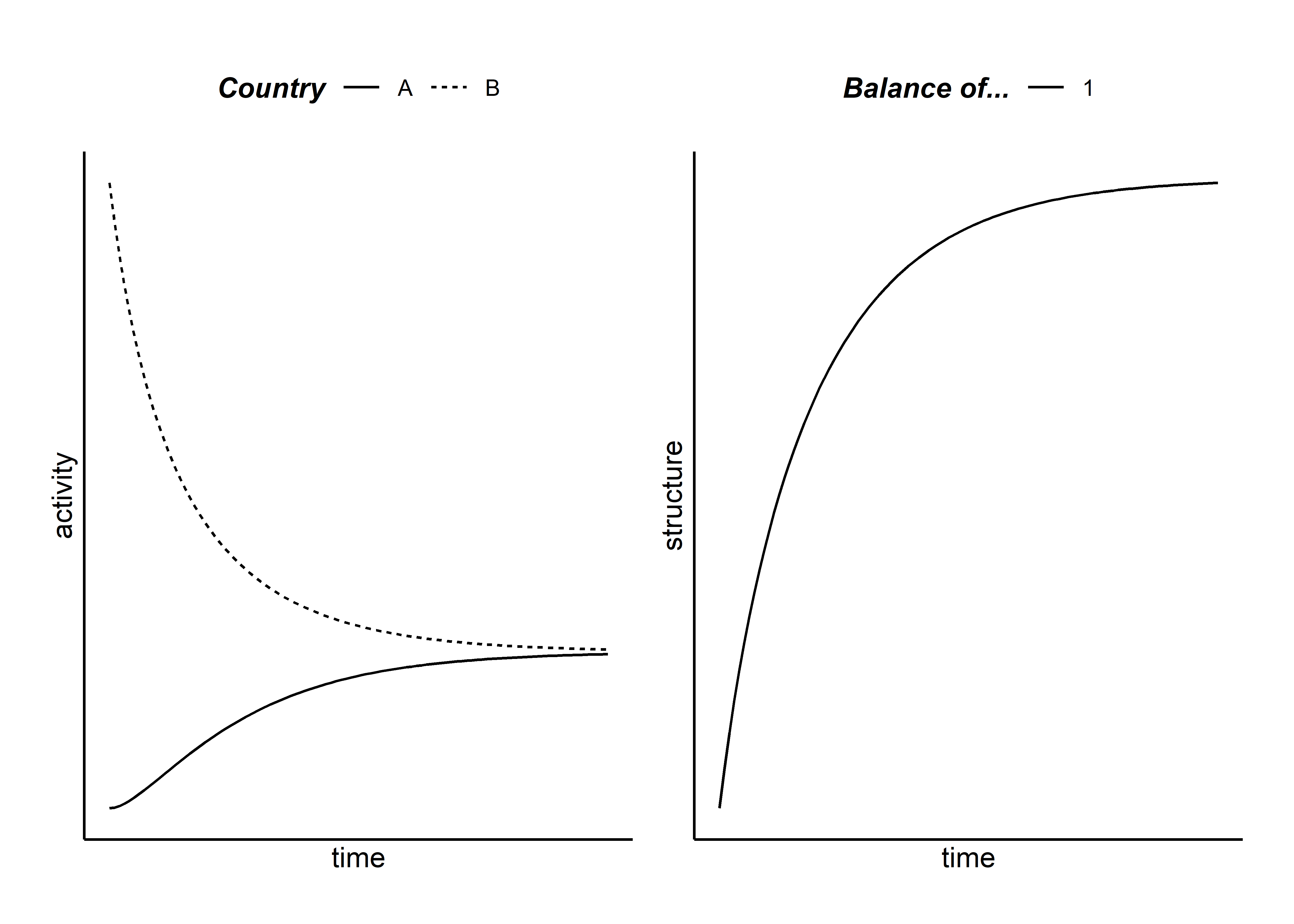
Given the starting parameters, the system moves closer to a balance between the preferences of country A and country B over time. As this happens, the former moves from being isolationist to more internationalist while the latter remains internationalist but with declining magnitude.
We can consider a more complex example, as well. Say we have a system with three countries and two dimensions characterizing the state of the world. These functions can easily generalize to this more complicated scenario.
## Define the starting parameters
w <- cbind(w1 = c(.5,.5), w2 = c(.7,.3), w3 = c(0.9, 0.1))
v <- cbind(i1 = c(1,1), i2 = c(0,0), i3 = c(0.3, 0.3))
s <- c(.3,.3)
p <- c(.7,.3, .1)
p <- p / sum(p)

## Let the system run
sys_out <- system(p=p,w=w,v=v,s=s)

## Plot the system over time
sys_plot(sys_out)

It’s that simple!
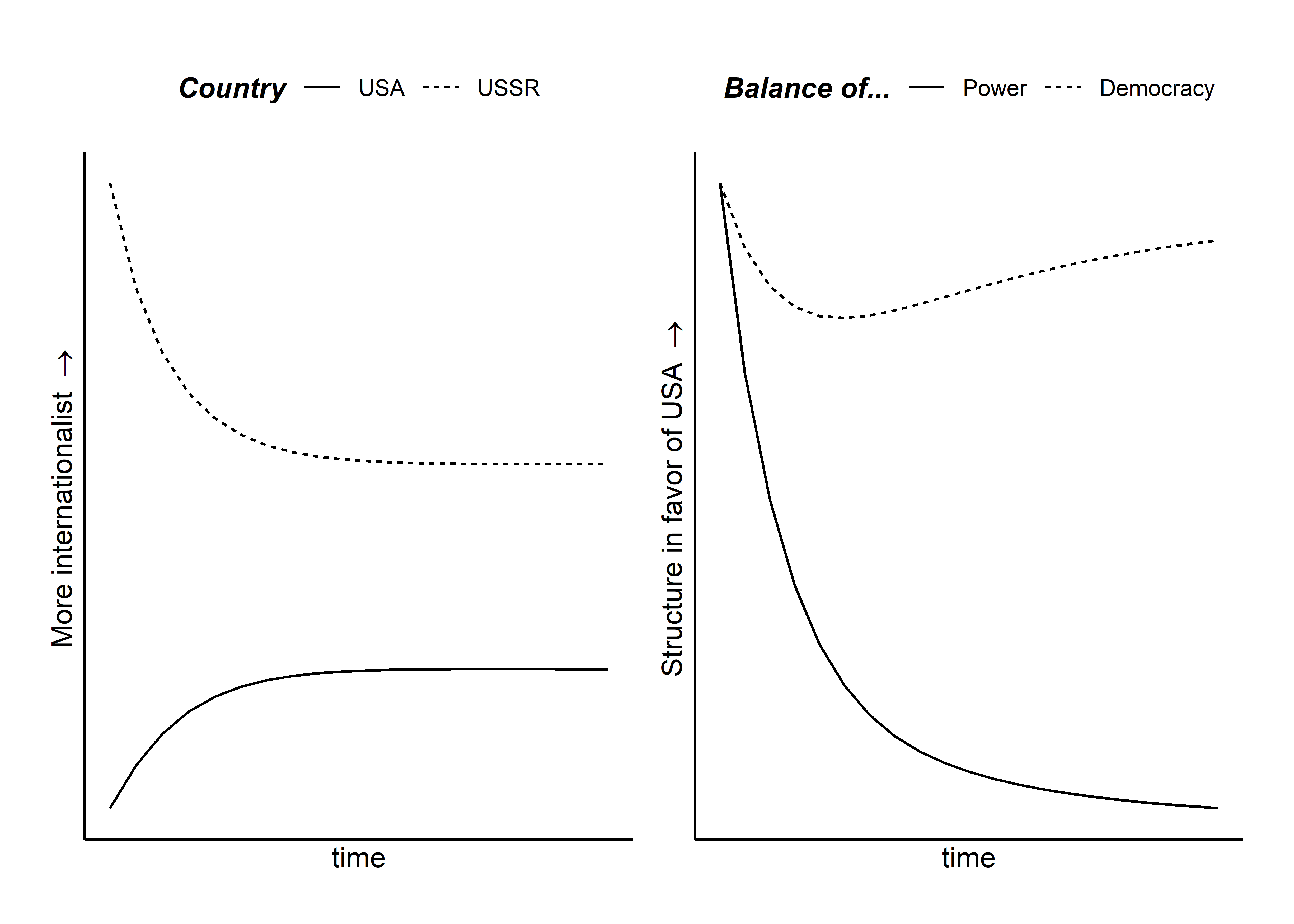
We can also update the labels. Say we wanted to just focus on the Cold War and have our countries be the US and the Soviet Union who are concerned about both the distribution of power and the distribution of ideology (democracy vs commumunism). We’ll assume both want all the power and only their preferred ideology to be adopted across the world. We’ll give the US more power and give it a 50/50 world view (it cares equally about power and ideology). The USSR will have less power and a world view that is slightly biased toward power (I don’t have a good historical justification for this choice, it just makes things interesting). We’ll start time with the US having an advantage in both dimensions of interest.
## Define the starting parameters
w <- cbind(w1 = c(.5,.5), w2 = c(.7,.3))
v <- cbind(i1 = c(1,1), i2 = c(0,0))
s <- c(.7,.7)
p <- c(.7,.3)

## Let the system run
sys_out <- system(p=p,w=w,v=v,s=s)

## Plot the system over time
sys_plot(sys_out,
         ylab = c(expression("More internationalist "%->%""),
                  expression("Structure in favor of USA "%->%"")),
         str.names = c("Power", "Democracy"),
         act.names = c("USA", "USSR"))
If this code is useful to you, please use it!