
Is an Insignificant Interaction Unimportant?
When it comes to hypothesis testing, I’m a sucker for a good interaction effect. But, I recently caught myself reflexively using the significance of interaction terms to adjudicate the conditionality of my hypothesis. When I thought about it a bit more I realized that an insignificant interaction is not the same thing as an unimportant one. This fact isn’t always obvious, so I thought I’d write a little something about it, both for my future self and for others out there using interaction terms but feeling low when the interaction isn’t different from zero.
Interaction terms answer two questions; not just one
I stumbled onto this piece published a few years ago in the Journal of World Business by Kingles, Noordewier, and Bergh (2017) on the topic of interaction terms. The authors note that when we estimate interaction effects, underlying those effects are two questions:
- Is there a statistically significant difference in the effect of the variable of interest given the conditioning variable?
- Is the effect of the variable of interest statistically different from zero given the conditioning variable?
When I think about interactions, question 1 is often what comes to mind. I want to see whether the variable I’m interested in has different effects given a conditioning factor.
I never really thought much (if at all) about question 2. At least I never thought about it explicitly, and that’s problematic. As Kingles, Noordewier, and Bergh (2017) note, ignoring question 2 can lead a researcher to prematurely discard a conditional hypothesis if the interaction term isn’t statistically significant—that is, if the answer to question 1 is no.
However, it is perfectly possible to have a scenario where the answer to question 1 is no but the answer to 2 is yes, and vice versa. Ignoring this leads to the problem of under- or overstating interaction terms, respectively. If we understate the interaction, we reject a conditional hypothesis solely on the basis of 1. If we overstate the interaction, we fail to reject a conditional hypothesis solely on the basis of 2 without considering whether the marginal effect of the variable of interest is different from zero given different values of the conditioning factor.
We should be answering both questions, and that means not only paying attention to the significance of the interaction but also to the variance of the marginal effect of interest given the condititioning variable.
A Simulation
A simulation will help. Let’s compare two data-generating processes or DGPs.
To start, we’ll work with an N of 1,000, a normally distributed explanatory variable of interest called X, and a binary conditioning variable called Z.
N <- 1000
X <- rnorm(N)
Z <- rbinom(N, 1, 0.5)
When we imagine interaction effects, I’d wager that we have something like the following in mind. The below code simulates a DGP for an outcome as Y = β0 + β1X + β2Z + β3X ⋅ Z. For convenience betas 0, 1, and 2 are set to zero. Notice that in the construction of the remaining, non-zero beta, that the magnitude is 1, but there’s some random heterogeneity thrown in the mix to create noise.
b1 <- 1 + rnorm(N)
Y1 <- b1 * X * Z + rnorm(N)
The above scenario implies that the effect of X when Z = 0 is 0 but 1 when Z = 1. The next scenario below is different. It defines a DGP where the average effect of X is constant given Z but where the variance in the effect is not.
b2 <- 1 + rnorm(N, sd = 1 + 5 * Z)
Y2 <- b2 * X + rnorm(N)
Now, if we estimate a pair of regression models for each of these outcomes and compare the results, we should see that for the first the interaction term for X and Z is positive and statistically significant. Meanwhile, the interaction term for the second is not.
library(estimatr)
fit1 <- lm_robust(Y1 ~ X * Z, se_type = "stata")
fit2 <- lm_robust(Y2 ~ X * Z, se_type = "stata")

## Compare
library(texreg)
screenreg(list(fit1, fit2), include.ci = F)
##
## =====================================
##              Model 1      Model 2
## -------------------------------------
## (Intercept)     0.03         0.08
##                (0.05)       (0.06)
## X              -0.07         0.90 ***
##                (0.04)       (0.09)
## Z              -0.00        -0.32
##                (0.08)       (0.30)
## X:Z             1.09 ***     0.08
##                (0.09)       (0.46)
## -------------------------------------
## R^2             0.25         0.04
## Adj. R^2        0.25         0.04
## Num. obs.    1000         1000
## RMSE            1.25         4.55
## =====================================
## *** p < 0.001; ** p < 0.01; * p < 0.05
Now be honest. If you saw the results as presented for model 2, what would you conclude? I admit that I’d jump to the conclusion that Z does not condition the effect of X on Y.
Not so fast! As Kingles, Noordewier, and Bergh (2017) remind us, we need to look at more than just whether the interaction is different from zero. We need to also check whether the marginal effect of the variable of interest is different from zero given the conditioning variable.
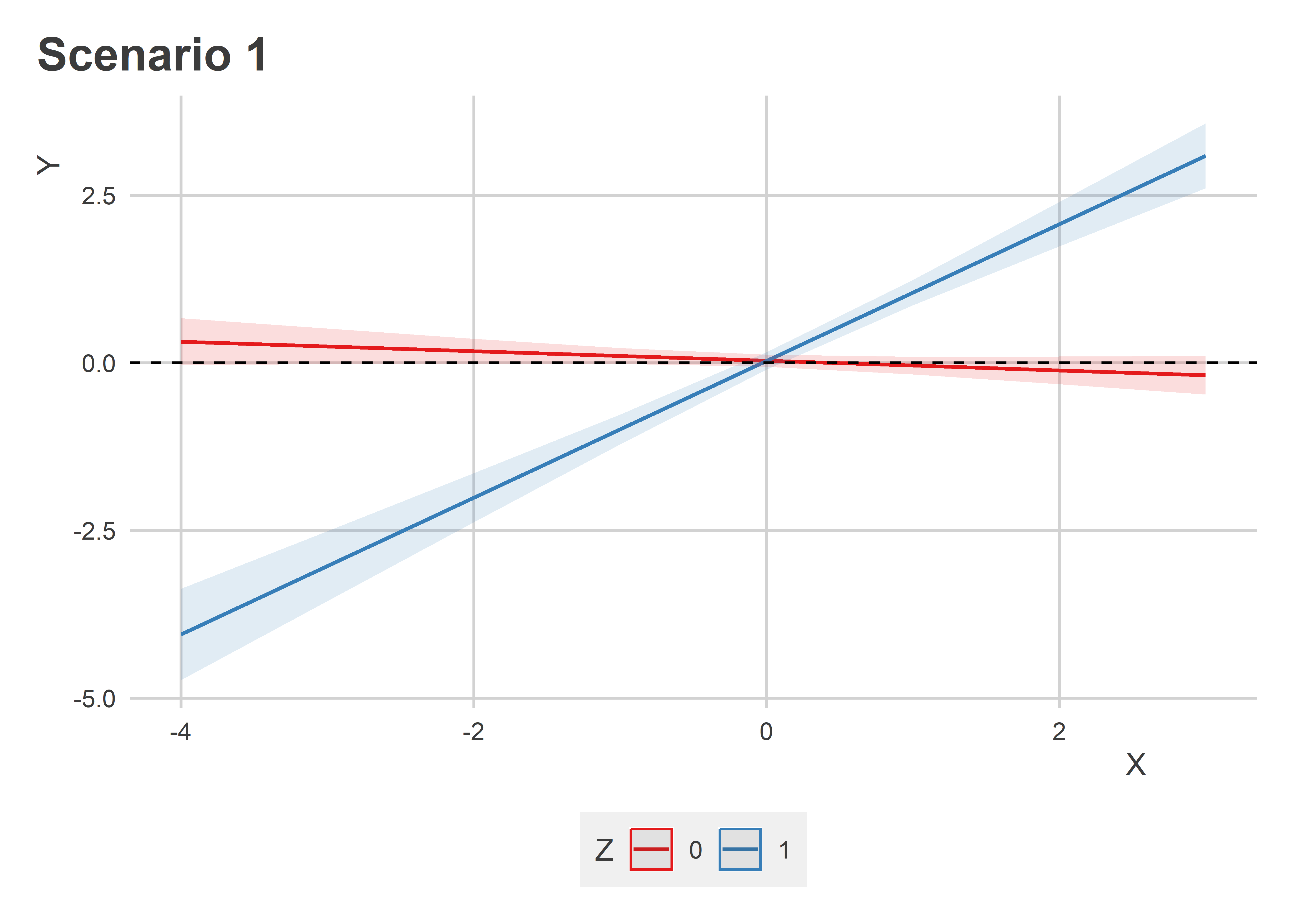
Simple interaction plots will suffice. The first below shows how the marginal effect of X changes given Z. The x-axis shows values of X, the y-axis shows predicted values of Y. Blue shows the effect of X when Z = 1 and red when Z = 0. Clearly, when Z = 0, X has no effect, but when Z = 1, X has a positive and statistically significant effect.
library(sjPlot)
plot_model(
  fit1,
  type = "int",
  terms = c("X", "Z")
) +
  labs(
    x = "X",
    y = "Y",
    title = "Scenario 1"
  ) +
  geom_hline(
    yintercept = 0,
    lty = 2
  )
This is not what we observe with the second model. The next figure shows how the effect of X on Y changes given Z in model 2. In this case, the slope of the effect of X is not statistically different given Z. But, whether the effect of X is statistically different from zero does change given Z.
plot_model(
  fit2,
  type = "int",
  terms = c("X", "Z")
) +
  labs(
    x = "X",
    y = "Y",
    title = "Scenario 2"
  ) +
  geom_hline(
    yintercept = 0,
    lty = 2
  )

Why care?
It’s incumbent on us researchers to think carefully about what our theories imply. In both of the scenarios above, we observe the same conditional implications for the effect of X given Z. When Z = 0, the effect of X on Y is not statistically different from zero. But, when Z = 1, the effect of X is different from zero. Do we care whether it also is the case that the marginal effect of X is statistically different given Z? Or is it immaterial to our theory? Sometimes the answer to the second question is “yes,” but we proceed as if the answer is “no” if we use the significance of the interaction term as a test of our conditional hypothesis.
I think I, and others as well, could do a better job of keeping these nuances in mind.