Something Is Amiss with the Log of Gravity

Back to Blog

In their seminal piece, Silva and Tenreyro (2006) made the case that PPML (Poisson Pseudo Maximum Likelihood) is a superior and robust method for estimating “gravity” equations compared to using OLS with a log-linear specification. I’ve received this advice myself, but before following it I thought it would be good to run a simple simulation to verify that the approach is all that it’s lauded to be.

To my surprise, and as I’ll detail below, I don’t find strong Monte Carlo evidence that PPML is the best way to model the “log of gravity.”¹

Why is PPML supposed to be better?

If you want the nitty gritty details about the superiority of PPML, I recommend reading the Silva and Tenreyro paper. The cliff notes version of it is this. There’s this thing called Jensen’s inequality which states E(lny) ≠ ln E(y). In words, the expected value, or mean of the natural log, of y is not equivalent to the natural log of the mean of y.

From an econometric perspective, what this implies is that the parameters of a log-linear model when estimated via OLS may be inconsistent in the presence of heteroskedasticity. But, if the model is estimated assuming a pseudo-poisson process this problem can be avoided—or so Silva and Tenreyro claim.

Is it actually better?

To test this claim, I used seerrr to generate some data based on a straightforward data-generating process. The standard gravity equation assumes a functional form for an outcome y that looks like:

y_i = exp (x_iβ)η_i,

which in log-linear form is equivalent to:

ln y_i = x_iβ + ln η_i.

In the above, x_i is a random variable and η_i is a log-normal stochastic term.

Taking this form as a cue, I simulated data for an outcome y_i as follows:

library(tidyverse) # for grammar
library(seerrr)    # for Monte Carlo experiments

# 500 random data simulates:
simulate(
  R = 500,
  eta = exp(rnorm(N, sd = runif(N, 0.5, 2))),
  x = rnorm(N),
  y = exp(0.5 * x) * eta
) -> sim_data

The error term in the above is specified as η_i = exp (𝒩[μ=0,σ_i²]) where the variance parameter is non-constant. The parameter β = 1/2 is the elasticity, or change in ln y given a unit change in x.

If PPML really is superior to OLS in the presence of non-constant variance, it should on average yield more consistent and efficient estimates of β. To check whether this is true, I first make a wrapper function that applies the quasipoisson option for glm. This is the method that packages such as gravity use under the hood to implement PPML.

ppml <- function(...) glm(..., family = quasipoisson)

I then estimate a log-linear model via OLS and the PPML model on the simulated data:

estimate( # log-linear OLS
  sim_data,
  log(y) ~ x,
  vars = 'x',
  se_type = 'classic'
) -> ols_fit
estimate( # poisson
  sim_data,
  y ~ x,
  vars = 'x',
  estimator = ppml
) -> ppml_fit

After running the above, we now have the following distribution of estimated βs obtained using each method:

bind_rows(
  ols_fit %>% 
    mutate(estimator = 'OLS'),
  ppml_fit %>%
    mutate(estimator = 'PPML')
) %>%
  ggplot() +
  aes(
    x = estimator,
    y = estimate - 0.5
  ) +
  geom_violin(
    draw_quantiles = c(0.025, 0.5, 0.975),
    fill = 'firebrick'
  ) +
  geom_hline(
    yintercept = 0,
    lty = 2
  ) +
  scale_y_continuous(
    breaks = 0,
    labels = 'Truth'
  ) +
  labs(
    x = 'Estimator',
    y = 'Elasticities',
    title = 'Is PPML better than OLS?',
    subtitle = 'Range of estimates from 500 simulations'
  )

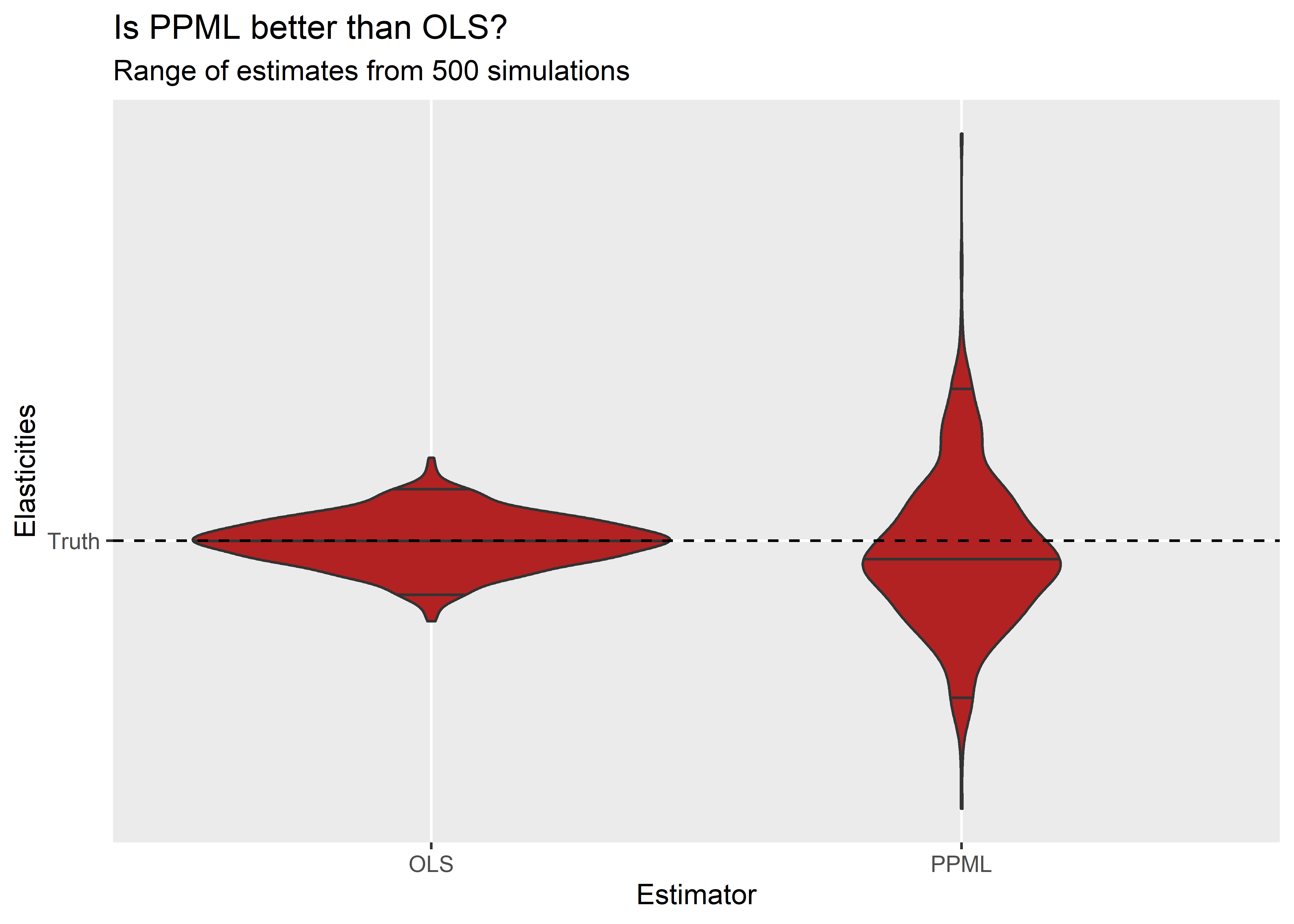
Much to my surprise, it seems that PPML provides a less consistent estimate of β than log-linear OLS. The above figure shows for the set of OLS estimates and PPML estimates the distribution of βs using a violin plot. The dashed horizontal line denotes the true parameter value, and the solid horizontal lines in the violin densities denote the 2.5, 50, and 97.5 percentiles of the simulated parameter estimates. It takes only a cursory examination of the figure to see that PPML yields a much wider dispersion of β estimates than OLS.

If we use the 'bias' option in the evaluate function, we can assess other characteristics of the OLS and PPML estimates:

bind_rows(
  evaluate(
    ols_fit, 
    what = 'bias',
    truth = 0.5
  ),
  evaluate(
    ppml_fit,
    what = 'bias',
    truth = 0.5
  )
) %>%
  mutate(
    estimator = c('OLS', 'PPML')
  ) -> eval

First, as we would expect given the range of estimates in the previous figure, the mean squared error (MSES) is substantially greater with PPML:

ggplot(eval) +
  aes(
    x = mse,
    y = estimator,
    label = round(mse, 3)
  ) +
  geom_col(
    width = 0.5,
    fill = 'firebrick',
    color = 'black'
  ) +
  geom_text(
    hjust = 1.2,
    color = 'white'
  ) +
  labs(
    x = 'Mean Squared Error',
    y = NULL,
    title = 'Is PPML better than OLS?',
    subtitle = 'Summary of 500 simulated estimates'
  )

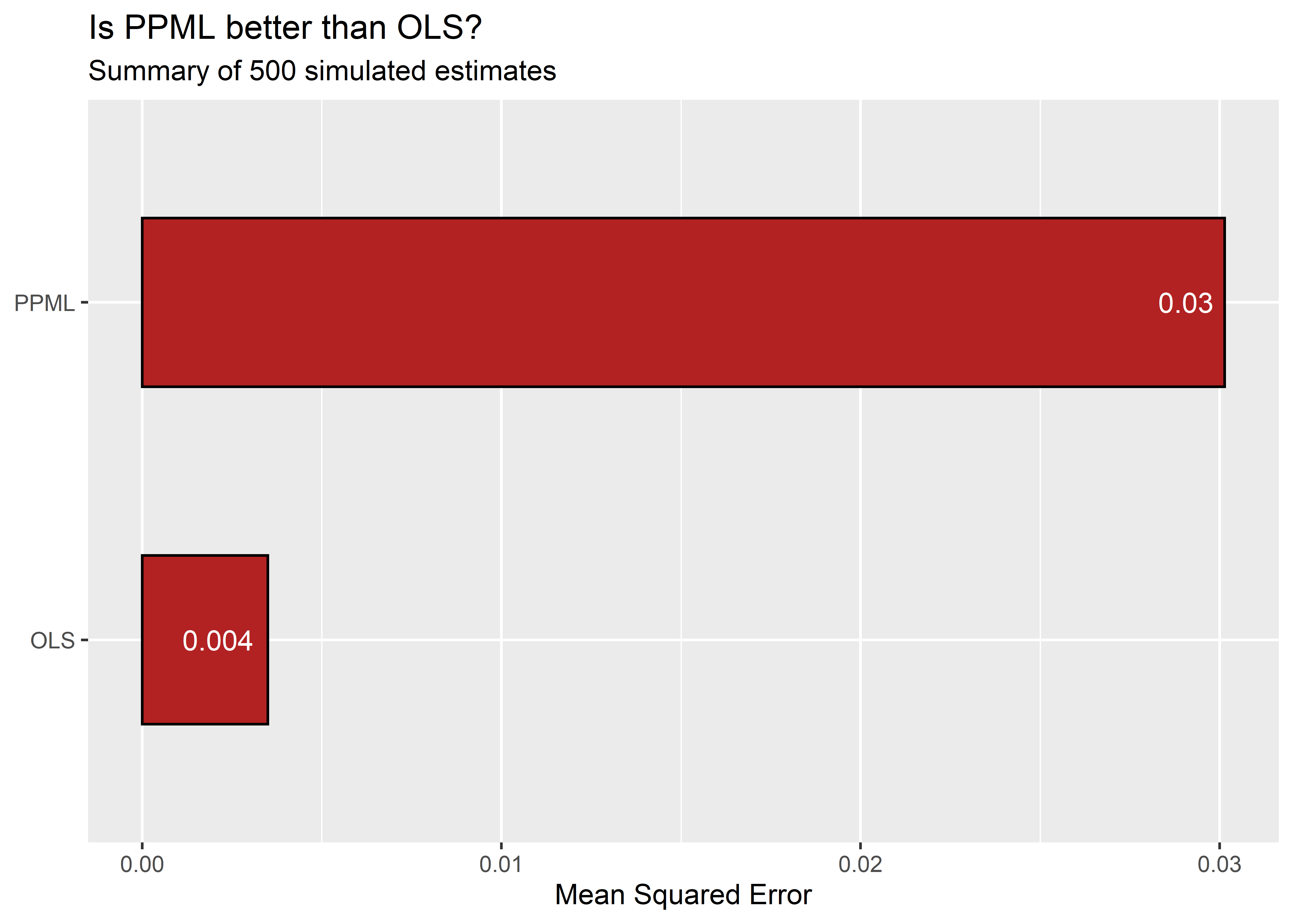
The above figure shows the MSE computed for the 500 simulated βs for both log-linear OLS and PPML using a bar plot. The MSE for the PPML estimator is several times greater than that for log-linear OLS.

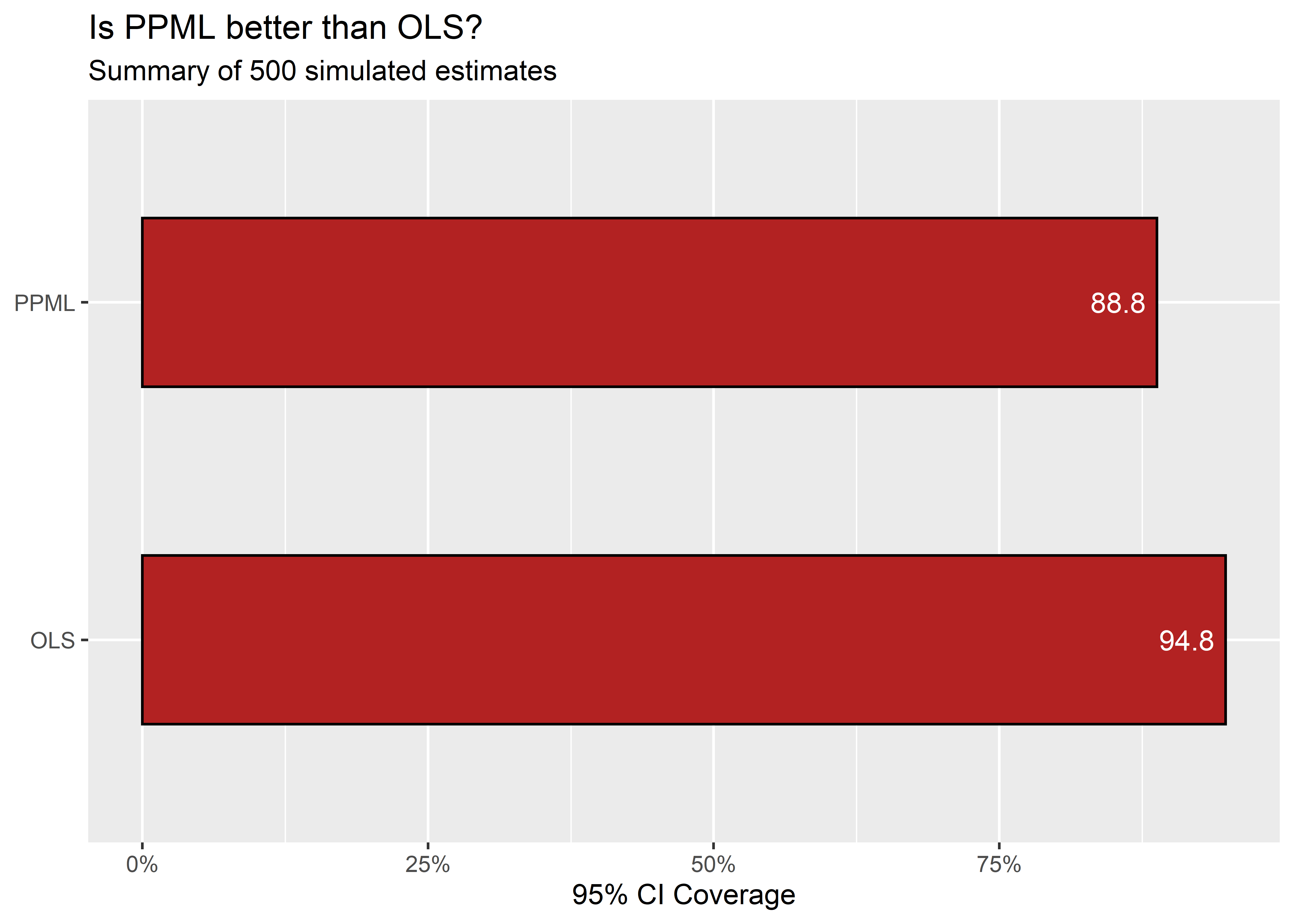
Not only is PPML less consistent, if we compare the coverage of the estimators’ 95% confidence intervals, despite the fact that PPML shows more variability than OLS (meaning it has on average larger standard errors), its coverage is deflated. The 95% CIs should contain the true parameter estimate on average 95% of the time with repeated samples. But PPML’s 95% CIs contain the true parameter value less than this amount while OLS 95% CIs have the appropriate coverage. This is shown in the next figure:

ggplot(eval) +
  aes(
    x = coverage,
    y = estimator,
    label = round(coverage * 100, 3)
  ) +
  geom_col(
    width = 0.5,
    fill = 'firebrick',
    color = 'black'
  ) +
  geom_text(
    hjust = 1.2,
    color = 'white'
  ) +
  scale_x_continuous(
    labels = scales::percent
  ) +
  labs(
    x = '95% CI Coverage',
    y = NULL,
    title = 'Is PPML better than OLS?',
    subtitle = 'Summary of 500 simulated estimates'
  )

What is to be done?

What to do in light of these unexpected findings is, to be fully transparent, unclear to me. The data-generating process I used in the above simulations is not the only realistic scenario so it probably is wise to avoid over-interpreting these results.

This exercise does, however, demonstrate how critical the design of Monte Carlo experiments is to the evaluation and comparison of alternative estimators. In this instance, specification of a fairly simple data-generating process yields findings contrary to those of Silva and Tenreyro. It probably should go without saying, but this is an important reminder that one-size-fits-all recommendations of appropriate estimators is ill-advised. Sometimes the law of gravity really is to take its log.

Back to Blog

Like the “law of gravity.” Get it? ↩