
Doing the Right Multinomial Test
[Note: There was an earlier version of this post that got a few things wrong (I’m only human). I’ve since corrected this.]
As a political scientist, I have to confess that something as basic as knowing how to properly apply a chi-squared test, and implement it correctly using statistical software, has been a blind spot for me. Linear regression, logit, and Tobit…no big deal. How difficult could a basic statistic like chi-squared be?
It turns out it can be pretty darn tricky. I learned this in the process of writing methods guidance for the US Office of Evaluation Sciences (OES). OES’s bread-and-butter research centers on embedding randomized controlled trials (RCTs) within existing or new US Federal Government policies. But lately, many projects have become more observational than experimental, with a significant subset of these projects being centered on identifying existing inequity in the disbursement of government benefits.
The analysts for one such project wanted to apply a chi-squared test to draw inferences about whether significant disparities exist between individuals who are eligible to receive certain financial benefits and individuals who actually receive these benefits. Their design involved tabulating the demographic profiles of these different groups and then applying a chi-squared test to determine if the differences observed between the recipient group and the eligible population are significantly different.
This idea seemed straightforward enough. Chi-squared tests are in a class of tests that are used to draw statistical inferences with respect to data that follow a multinomial distribution.
The goal is simple. Suppose we have a dataset with individuals divided into two groups. In group A we have individuals who voted in a US mid-term election. In group B we have those who did not. For simplicity’s sake, assume the only demographic variables we have for individuals in each group are gender (F = 1 if female, 0 if male) and whether an individual has at least a four-year degree (D = 1 if yes, 0 otherwise).
For each of the groups, there are four unique strata into which individuals can fall:
- Female and a four-year degree (F = 1 and D = 1);
- Female and no degree (F = 1 and D = 0);
- Male and a four-year degree (F = 0 and D = 1);
- Male and no degree (F = 0 and D = 0).
The frequency distributions of each strata differ between groups. As the below figure summarizes, women and those with a four-year degree are over-represented among voters (group A) and are under-represented among non-voters (group B).
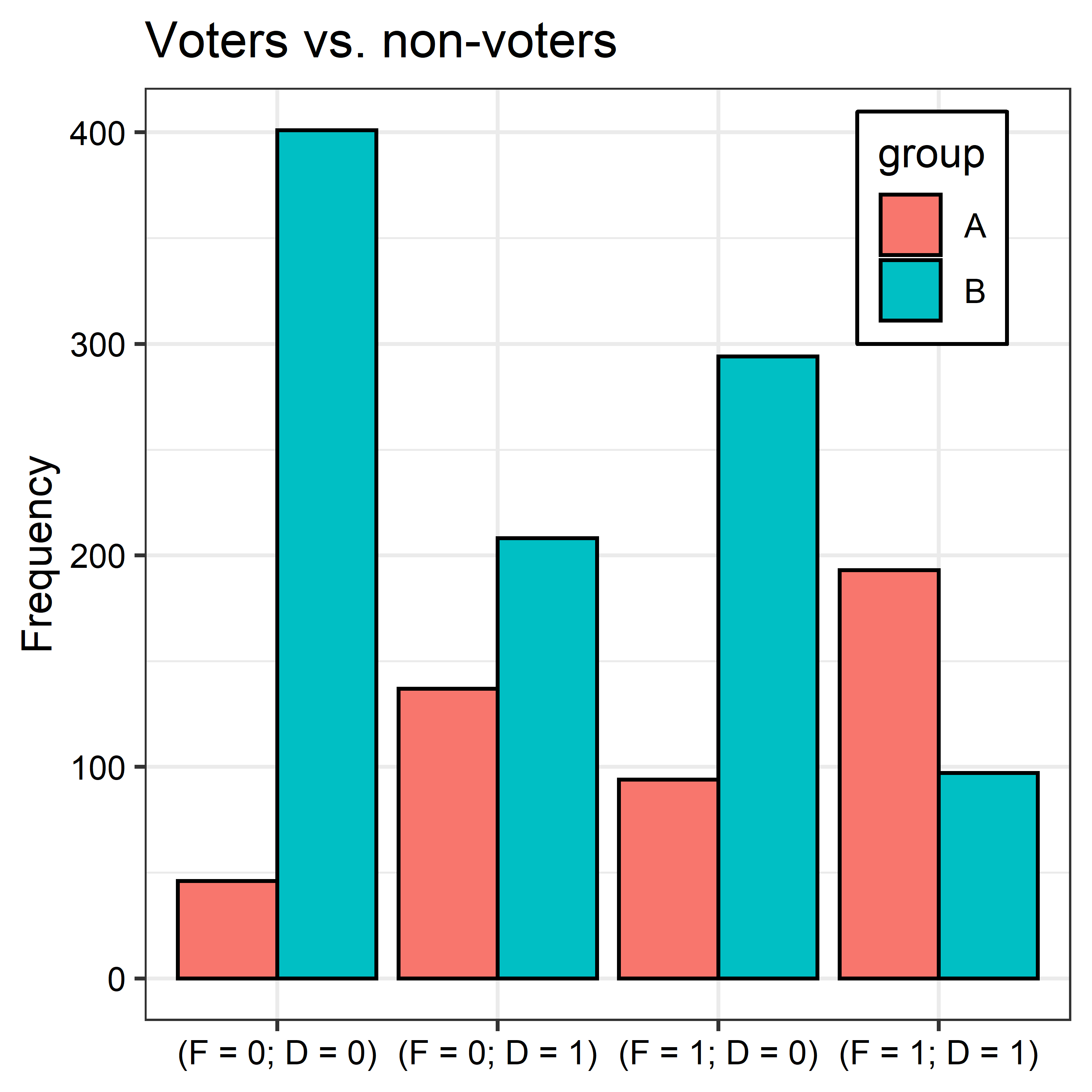
The groups clearly look different, but is this difference statistically detectable? We can answer this question using a multinomial test, such as chi-squared:
# perform chi-squared test
chisq.test(
  x = cbind(
    dt$freq[1:4],
    dt$freq[5:8]
  )
)
##
##  Pearson's Chi-squared test
##
## data:  cbind(dt$freq[1:4], dt$freq[5:8])
## X-squared = 276.24, df = 3, p-value < 2.2e-16
The output shows the computed chi-squared statistic with its p-value, which is well below the usual 0.05 threshold, meaning we can reject the null that the sub-populations are drawn from the same multinomial distribution. In other words, voters and non-voters are different.
The Problem
So, all seems good. Right? The convenience of a multinomial test in this context is its relatively few assumptions. It simply lets us consider whether the frequencies in each strata between groups A and B are too different from one another to be the result of chance. Beyond this, it makes no assumptions about the form or direction of this difference. This is a good justification for using this kind of test for addressing questions like that posed above, or in particular questions related to equity like the OES project I mentioned above.
However, as it turns out, the way the team of OES analysts wanted to use the chi-squared test started to look problematic to me.
I love to tinker with things, and I started to run simulations to get some power and false-positive rate calculations for chi-squared tests (because that’s what normal people do, right?). I didn’t expect anything weird to come out of this exercise—maybe some anti-conservative bias in asymptotic versions of the test relative to Monte Carlo versions, but nothing major.
Much to my surprise, I noticed something really unusual. In in several simulations I was finding 30% false-positive rates! For reference, a properly performing test should have a false-positive rate of 5%. This was bad.
At first, I thought there might be a pathology associated with multinomial tests related to the multiple comparisons problem. Unlike a t-test, I thought, which considers the likelihood that the difference in means of two groups is greater than we’d expect by chance, a multinomial test like chi-squared considers differences across multiple strata between groups. In the case of the voting example above, four comparisons are being made on the basis of voting status—not just one.
This would be problematic from a testing perspective because as the number of statistical tests being considered grows, the likelihood of falsely rejecting the null hypothesis increases (this is the multiple comparisons problem in a nutshell).
After going down the rabbit-hole on this line of thinking, and pouring time into writing OES guidance (and a previous version of this post), a colleague of mine at OES (who also had not spent much time in the weeds with chi-squared tests) came across some statistical materials detailing different kinds of chi-squared tests.
It turns out you can implement what’s called a goodness of fit (GOF) chi-squared test or a chi-squared test of independence. The folks at OES (and me!) had been operating as if the first kind of test was the only test to use. In fact, we should have been using the other kind of test.
Chi-squared Tests
GOF tests and independence (IND) tests are suited to one of two scenarios respectively:
- If we want to draw inferences about whether a sample was drawn from a population or well-defined multinomial data-generating process, we should use a GOF test.
- If we want to draw inferences about whether two samples were drawn from the same multinomial data-generating process, we should use an IND test.
I’ll use an example with dice to illustrate.
Is a die fair?
First, suppose we want to determine if a six-sided die is fair or biased. With a fair die, the probability of rolling any individual number should be p = 1/6. There are six sides, and if the die isn’t biased, then the probability that we roll 1, 2, 3, etc. should be 1 out of 6.
We can “make” a six-sided die in R by writing a simple function called
(most originally) die(...):
die <- function() sample(1:6, size = 1)
die() # test run ("roll")!
## [1] 1
By design, since this function is a wrapper for the sample() function
the die function should be unbiased (or fair). If we roll it 100 times,
for example, it should be the case that the proportion of times a 1, 2,
3, all the way up to 6 is rolled is roughly 1/6.
We can check this in R by writing:
# Roll the die 100 times
rolls <- 100
observed_rolls <- replicate(
  rolls, die(), 'c'
)

# Visualize the output and compare to the expected
# distribution
library(tidyverse)
tibble(
  side = as.factor(rep(1:6, len = 12)),
  proportions = c(
    table(observed_rolls) / 100,
    rep(1/6, len = 6)
  ),
  label = rep(
    c('Observed', 'Expected'),
    each = 6
  )
) %>%
  ggplot() +
  aes(
    x = side,
    y = proportions,
    fill = label
  ) +
  geom_col(
    color = 'black',
    position = position_dodge()
  ) +
  geom_hline(
    yintercept = 1/6,
    lty = 2
  ) +
  scale_fill_manual(
    values = c('firebrick','darkblue')
  ) +
  labs(
    x = 'Sides of the Die',
    y = 'Proportion of Times Rolled',
    fill = NULL,
    title = 'Is the die fair?',
    subtitle = 'Expected vs. observed proportions after 100 rolls'
  ) +
  theme_light()
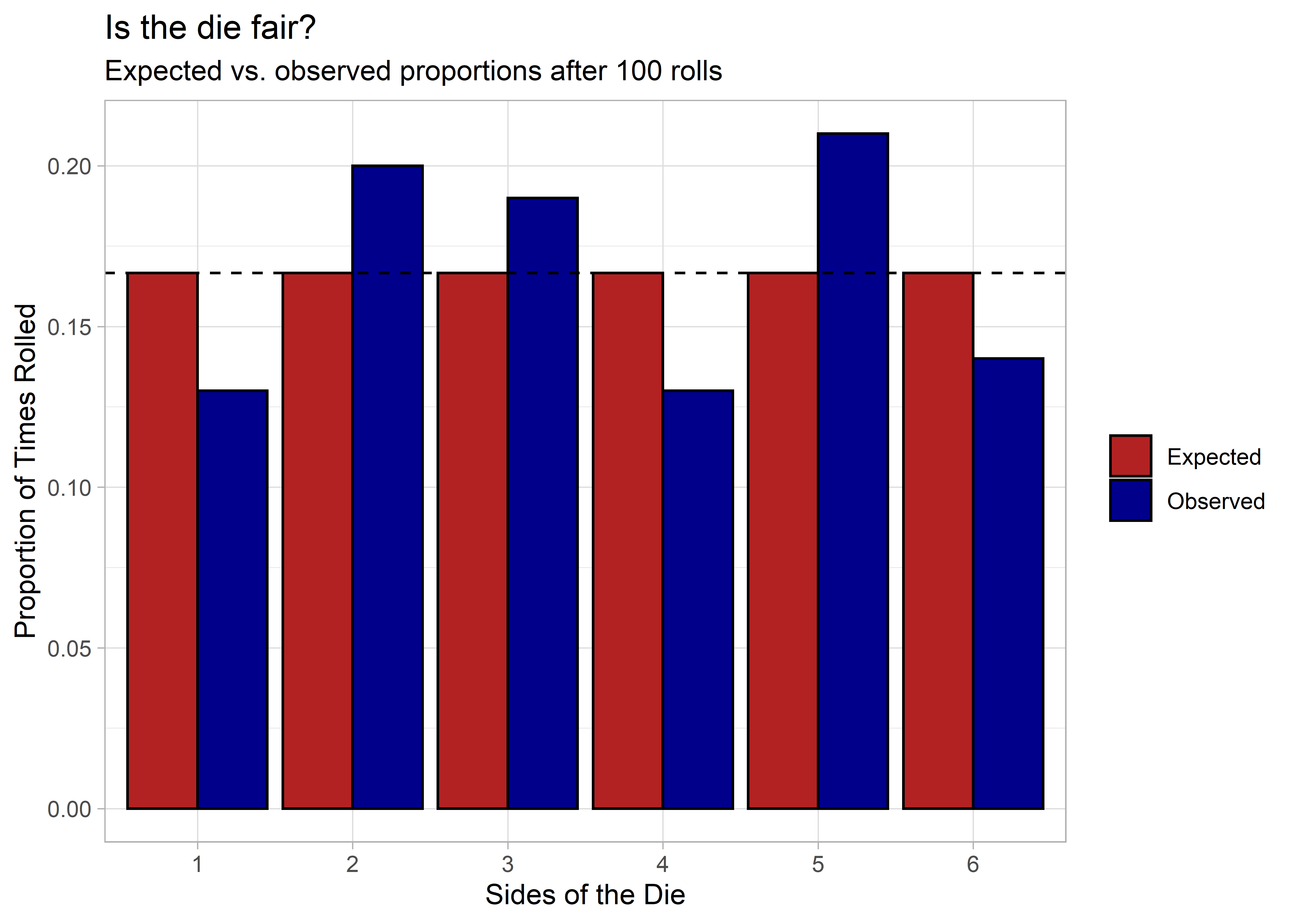
It looks mostly fair. There’s some variation, which is to be expected, but nothing so drastic to alert us to anything wrong with the die.
But just to be sure, we can get some help from our friend the chi-squared GOF test. We can implement this in R as follows:
x <- table(observed_rolls)
p <- rep(1/6, len = 6)
chisq_out <- chisq.test(x = x, p = p)
chisq_out # the chi-squared results
##
##  Chi-squared test for given probabilities
##
## data:  x
## X-squared = 4.16, df = 5, p-value = 0.5266
We have a p-value of 0.53, which is well above the conventional p < 0.05 significance threshold. In short, we can’t reject the null hypothesis that the die is fair.
Are two dice equivalent?
Testing whether a die is fair is simple enough. What about testing if two dice are equivalent?
To answer this question we need a modified version of the chi-squared test. Unlike in the previous example where we were comparing tabulated frequencies from a sample to expected frequencies, now we will be comparing tabulated frequencies from two different samples.
This means there are now two sources of uncertainty we need to account for in our test. In the previous example, we only needed to account for one source of uncertainty.
To illustrate, let’s make a new die function and compare it to the old one:
# Make a new die function
new_die <- function() sample(1:6, size = 1)

# Roll this die and the old die 100 times
rolls <- 100
old_die_rolls <- replicate(rolls, die(), 'c')
new_die_rolls <- replicate(rolls, new_die(), 'c')

# Visualize to compare
tibble(
  sides = as.character(rep(1:6, len = 12)),
  rolls = c(
    table(old_die_rolls),
    table(new_die_rolls)
  ),
  label = rep(
    c('Old', 'New'), each = 6
  )
) %>%
  ggplot() +
  aes(
    x = sides,
    y = rolls,
    fill = label
  ) +
  geom_col(
    color = 'black',
    position = position_dodge()
  ) +
  scale_fill_manual(
    values = c('firebrick','darkblue')
  ) +
  labs(
    x = 'Sides of the Dice',
    y = 'Frequencies',
    fill = 'Die',
    title = 'Are two dice equivalent?',
    subtitle = 'Observed frequencies for two dice after 100 rolls each'
  ) +
  theme_light()
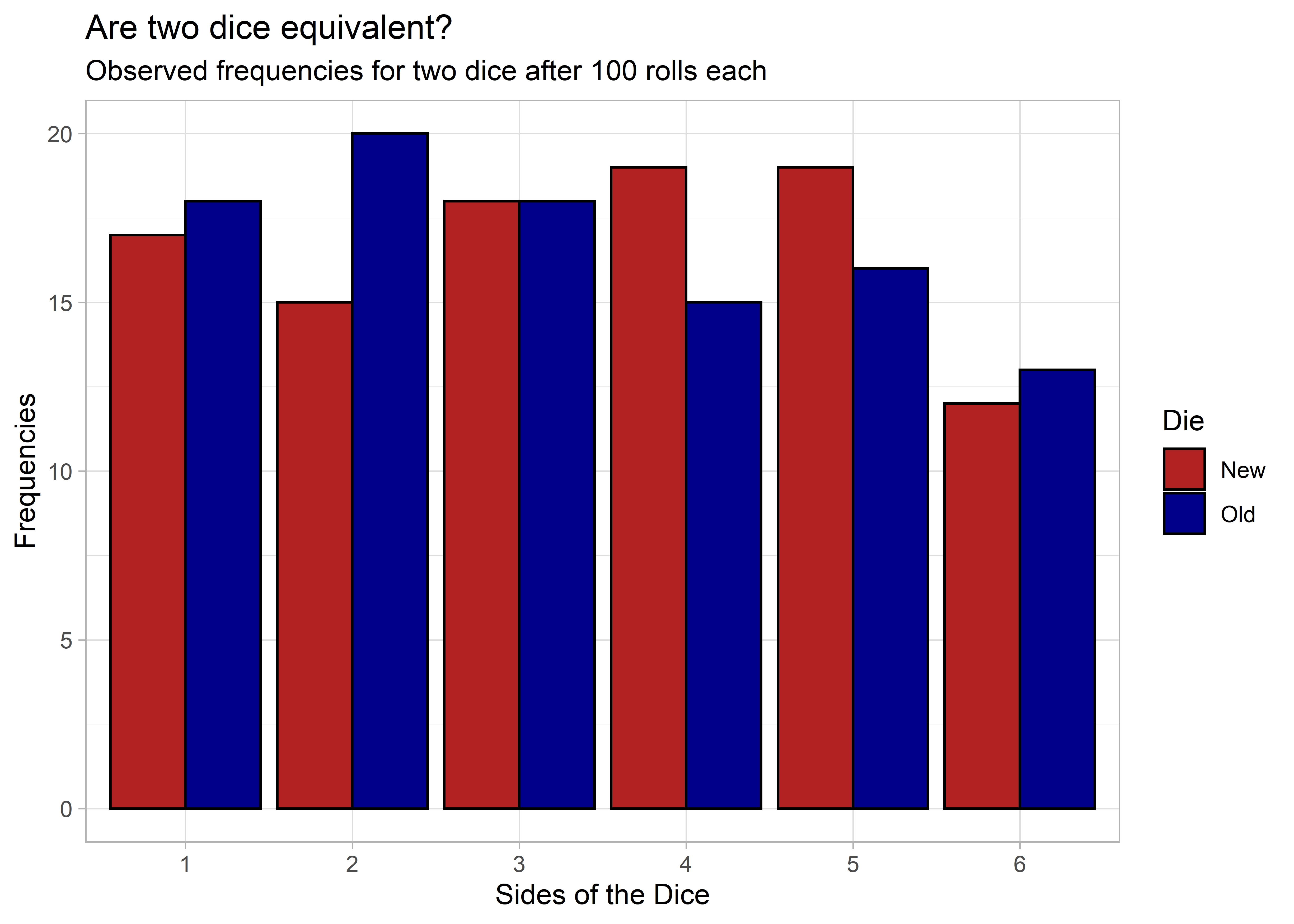
As we would expect, there’s some variation between the dice, but that’s normal when dealing with observed data.
If we want to be sure, we can implement an IND test in R to check:
# We need to put the data in a 2-dimensional array:
X <- cbind(
  old_die = table(old_die_rolls),
  new_die = table(new_die_rolls)
)

# Then we do the chi-squared test like so:
chisq_out <- chisq.test(x = X)
chisq_out # look at the output
##
##  Pearson's Chi-squared test
##
## data:  X
## X-squared = 1.5106, df = 5, p-value = 0.9118
Even though we observed some differences in frequencies, these differences are not statistically significant. The p-value is 0.91, which is well above the usual p < 0.05 significance threshold.
Getting our wires crossed
It’s pretty simple. Use GOF tests when comparing a sample to a population, and use an IND test when comparing two (or more) samples with each other.
While this advice is straightforward enough, it is surprisingly easy to misapply these tests—as in the case of the OES project I mentioned above that deals with equity. The analysts for that project wanted to use a GOF test, but this choice ignored the fact that the eligible group of beneficiaries was a sample—not the full population.
When we misapply the GOF test like this, we run into the problem that I had identified in simulations with this test: a really high false-positive rate.
To illustrate, suppose we took the same two dice compared above and rather than perform an IND test to determine if the two dice are equivalent we performed the GOF test and treated one of the dice as a referent group that captures the expected frequencies of the other die.
# Roll the dice
rolls <- 100
old_die_rolls <- replicate(rolls, die(), 'c')
new_die_rolls <- replicate(rolls, new_die(), 'c')

# Apply the GOF test rather than IND test
x <- table(new_die_rolls)
p <- table(old_die_rolls) / 100
chisq_out <- chisq.test(x = x, p = p)
chisq_out
##
##  Chi-squared test for given probabilities
##
## data:  x
## X-squared = 12.601, df = 5, p-value = 0.02742
If we run the GOF test, we get a chi-squared statistic and a p-value—with no objection from R, by the way!
It may be hard to tell just from looking at the results from one run of the test that there’s a problem here. But, if we run the test a bunch of times and collect the p-values from each run of the test, we can see the problem quite clearly.
The below code repeats what the above script does 1,000 times and collects the p-values.
its <- 1000

run_the_test <- function() {
  rolls <- 100
  old_die_rolls <- replicate(rolls, die(), 'c')
  new_die_rolls <- replicate(rolls, new_die(), 'c')

  # Apply the GOF test rather than IND test
  x <- table(new_die_rolls)
  p <- table(old_die_rolls) / 100
  chisq_out <- chisq.test(x = x, p = p)
  chisq_out$p.value # return the p.value
}

p.values <- replicate(its, run_the_test(), 'c')
head(p.values) # we have a collection of p-values
## [1] 0.0047789999 0.0012484284 0.0003859263 0.0581451295 0.6902624535
## [6] 0.2705798451
If the test is performing as it should, we should get p-values less than 0.05 about 5% of the time. But this isn’t the case:
fpr <- round(100 * mean(p.values <= 0.05), 2)
cat('The test rejects the null ', fpr, '% of the time.', sep = '')
## The test rejects the null 38% of the time.
This is way too liberal! If we look at the distribution of p-values, we can see what the problem is:
ggplot() +
  geom_histogram(
    aes(x = p.values),
    color = 'black',
    fill = 'firebrick'
  ) +
  labs(
    x = 'p-values',
    y = 'Frequencies',
    title = 'The null-distribution of p-values',
    subtitle = 'When the GOF test is inappropriate we get a\nskewed p-value distribution'
  )
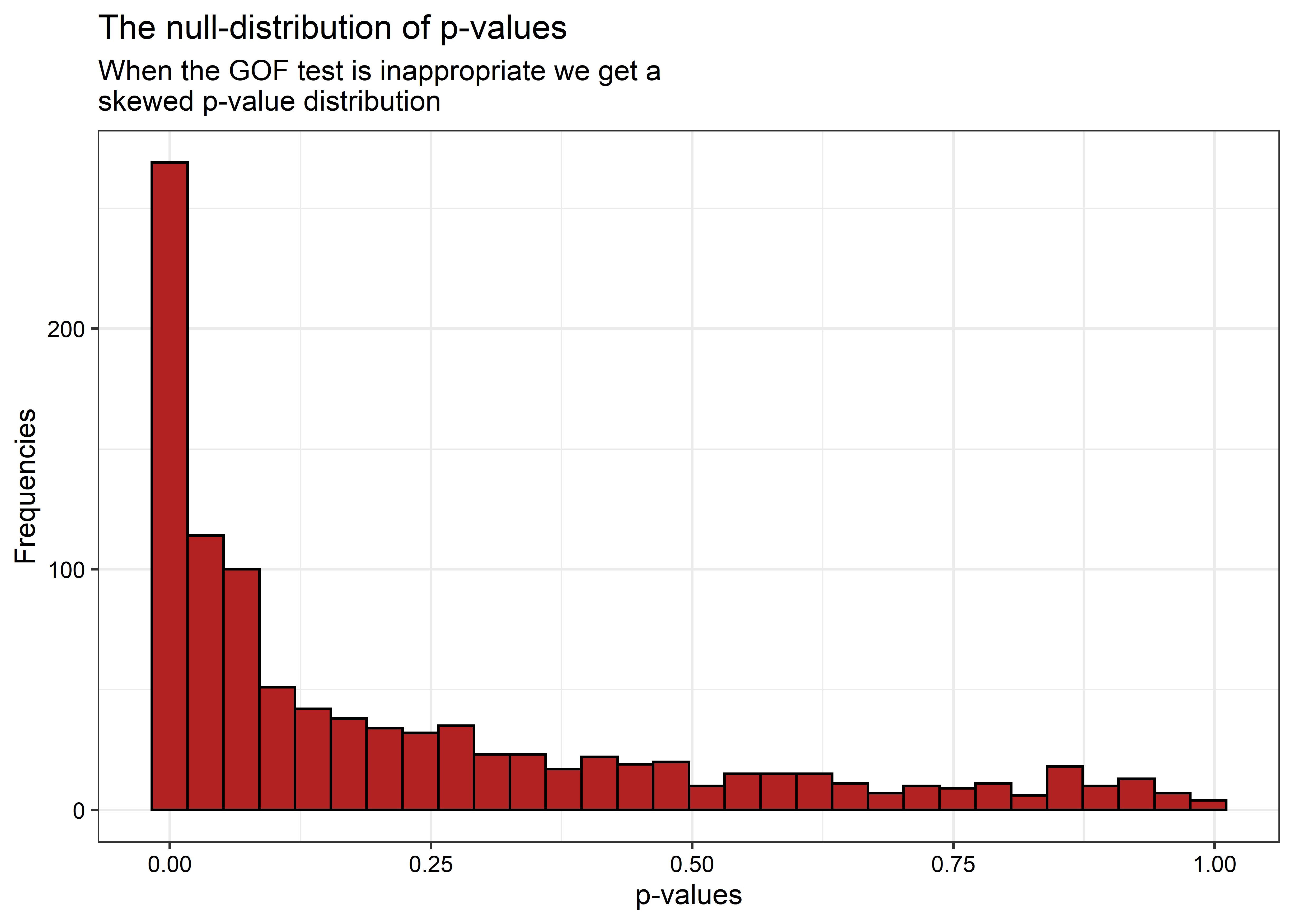
When the null hypothesis is true (and it is in this case, because the new and old die functions do exactly the same thing), this distribution should be uniform.
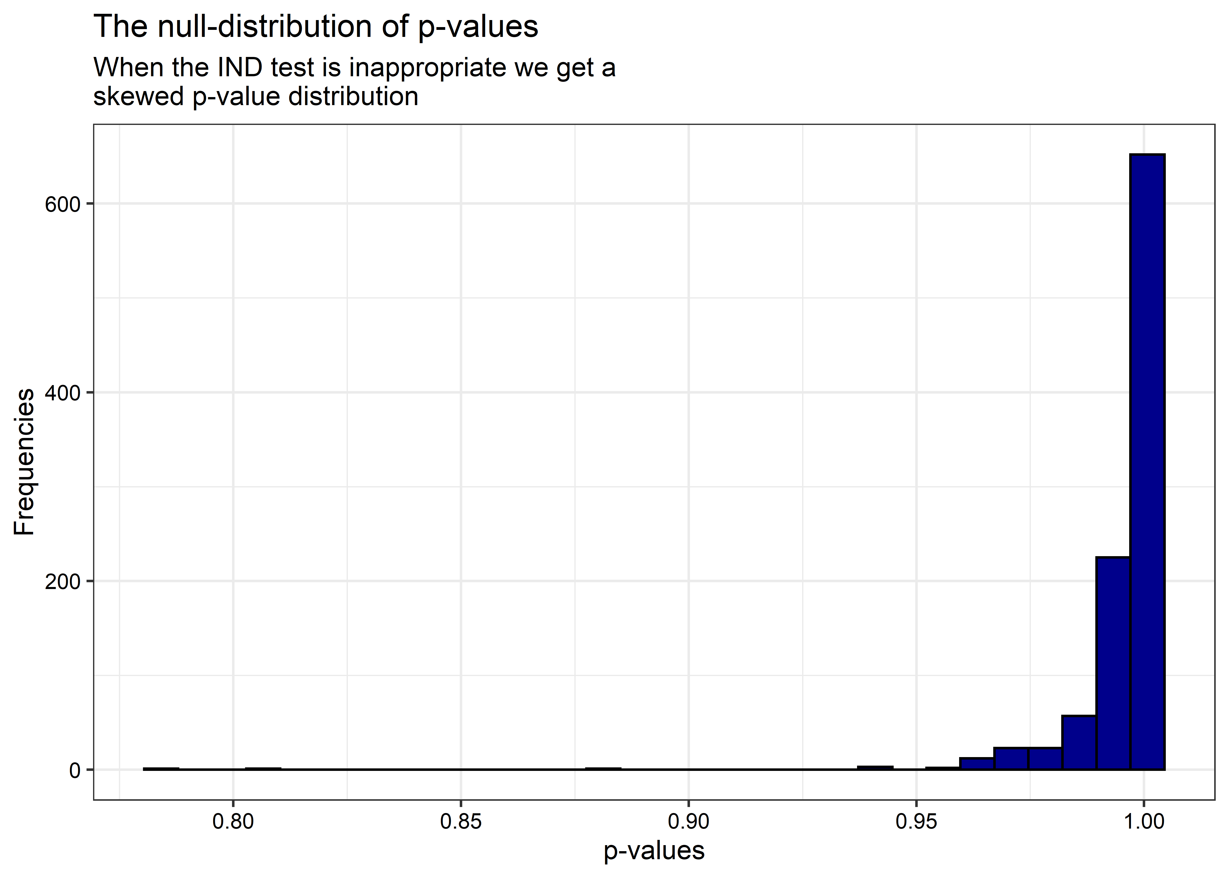
We get the reverse problem if we mistakenly use the IND test when the GOF would be appropriate. If we repeat the simulation again, but this time use the IND test to determine if a single die is fair, we’ll get a very small false-positive rate.
its <- 1000

run_the_test <- function() {
  rolls <- 100
  die_rolls <- replicate(rolls, die(), 'c')
  expected_rolls <- rep(1/6) * rolls

  # Apply the IND test rather than GOF test
  X <- cbind(
    table(die_rolls),
    table(expected_rolls)
  )
  chisq_out <- chisq.test(x = X)
  chisq_out$p.value # return the p.value
}

p.values <- replicate(its, run_the_test(), 'c')
head(p.values) # we have a collection of p-values
## [1] 0.9880163 0.9997558 0.9948830 0.9960407 0.9997743 0.9904693
The false-positive rate is basically zero now:
fpr <- round(100 * mean(p.values <= 0.05), 2)
cat('The test rejects the null ', fpr, '% of the time.', sep = '')
## The test rejects the null 0% of the time.
And the distribution of p-values is now skewed in the opposite direction:
ggplot() +
  geom_histogram(
    aes(x = p.values),
    color = 'black',
    fill = 'darkblue'
  ) +
  labs(
    x = 'p-values',
    y = 'Frequencies',
    title = 'The null-distribution of p-values',
    subtitle = 'When the IND test is inappropriate we get a\nskewed p-value distribution'
  )
Conclusion
The moral of the story is: use the right test for the question you want to ask! This is incredibly important, not just for making sure the dice for your favorite board game are working properly, but also for making sure that a much needed Federal government benefit is being distributed equitably.
If you’re comparing a sample to a population, Do a goodness of fit test.
If you’re comparing a sample with another sample, Do a test of independence.
Q.E.D.