
The Origin and Counterfactuals
Causal inference requires identifying an appropriate counterfactual—what a variable on a unit of observation would look like under an alternative condition of some causal variable.
However, we can’t actually observe counterfactuals, which is the fundamental problem of causation. Instead, we often take either a scientific or statistical approach to causal inference. In the former, the counterfactual is an identical unit to the one being manipulated by some intervention—either the unit itself before intervention or one identical to said unit in every way possible.
The latter approach, which is the one we most often take in the social sciences, involves collecting data on lots of units of observation and taking steps to make units as comparable as possible. Most often, we do this with a regression model that may include observed covariates we want to adjust for in our analysis.
I don’t want to discuss this approach in its entirety. Instead, I want to zero in on an important mechanical feature of regression analysis: how it synthesizes a counterfactual from lots of data points so we can identify a causal effect.
The Origin Is the Counterfactual
Suppose we have two variables, x and y that we observe on five individuals. To keep things simple let x and y be normal random variables.
Say we want to know the effect of x on y. The below figure plots y over x, after mean centering each, on a simple Cartesian plane. I’ve also overlaid a set of lines, each with zero as its intercept, that intersect with each point.
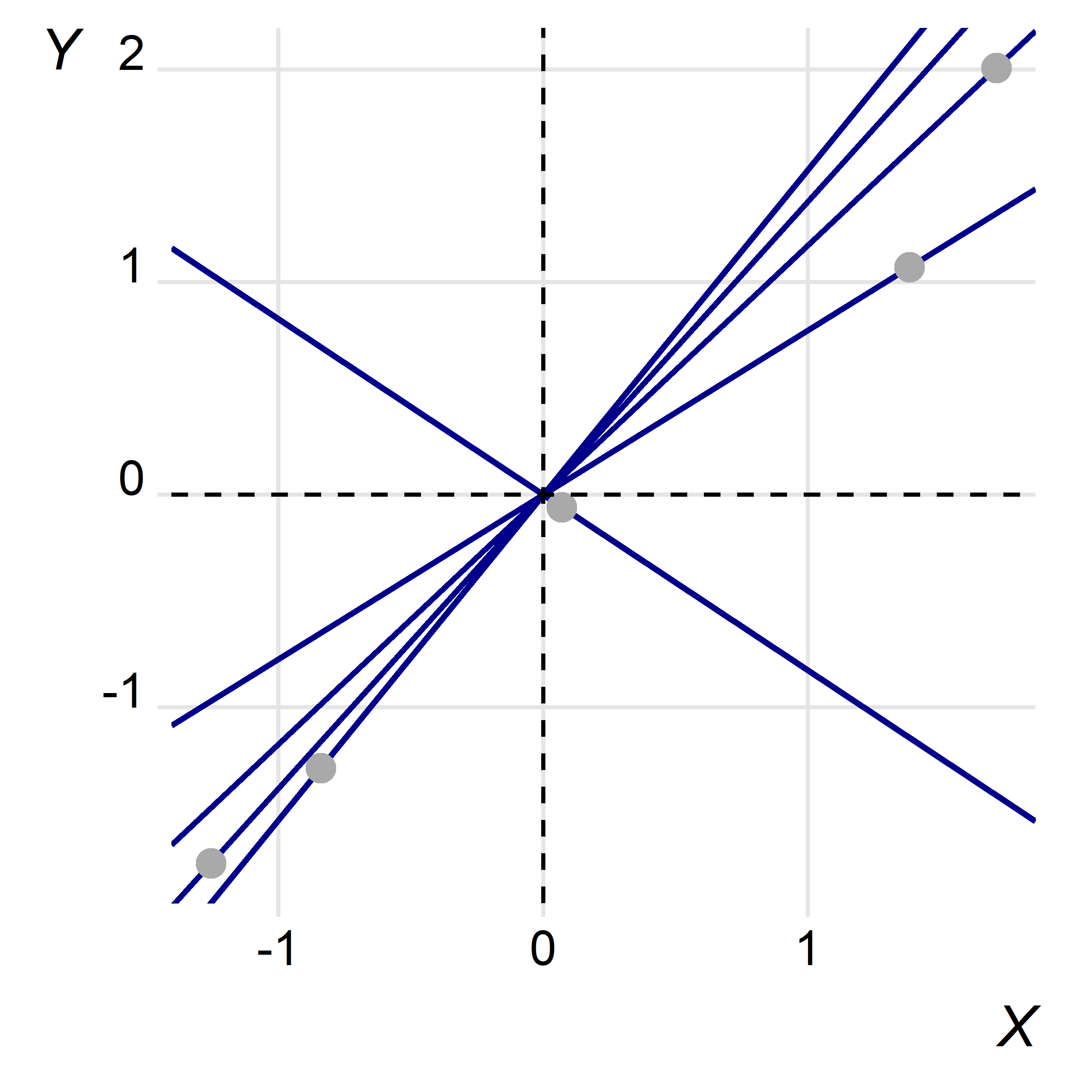
When we want to know the slope of a line we simply take its rise over its run. In this case, the slope for observation i is just yi/xi and the origin of the Cartesian plane is the referent point (the point where both x and y equal zero).
When we estimate a linear regression model the coefficient on the variable of interest will come from a coordinate space much like the one depicted here. The fitted regression will be the weighted average of the individual slopes per each unit of observation—and, for each observation the origin of the Cartesian plane will serve as the reference point, the spoke out of which each observation’s slope radiates.
Now, the fitted regression line, while it takes into account each of the individual slopes, is not just their raw average. Rather, it is a weighted average of the slopes, where the weights are proportional to the squared distance of the mean-centered predictor variable from the origin.
We can see this using the dummy data I created to generate the above figure:
# OLS coefficient:
b <- lm(y ~ x, dat) %>% coef %>% .["x"]

# Avg. Slope
s <- with(dat, mean((y - mean(y)) / (x - mean(x))))

# Function to recover weighted mean of slopes:
#   - to mean center a variable:
demean <- function(x) x - mean(x)
#   - to get the weighted mean of a variable:
wtmean <- function(x, wt) sum(wt * x) / sum(wt)
#   - to compute the regression line:
wtslope <- function(x, y) {
  mx <- demean(x)
  my <- demean(y)
  wt <- mx^2
  slope <- wtmean(my/mx, wt)
}

# The weighted mean slope:
ws <- with(dat, wtslope(x, y))

# Compare:
tibble(
  "OLS" = b,
  "Mean Slope" = s,
  "Weighted Mean Slope" = ws
)
## # A tibble: 1 x 3
##     OLS `Mean Slope` `Weighted Mean Slope`
##   <dbl>        <dbl>                 <dbl>
## 1  1.18         1.01                  1.18
We can see from the above that the weighted average of the individual slopes is identical to that recovered using OLS. For good measure, I’ve shown what we would get if we just took the raw average of the slopes. The estimate is close, but not equal, to the OLS estimate.
A similar thing happens when we estimate a multiple regression model, but the appropriate weights and the location of points around the origin will be different. This is because in a multiple regression model values of another variable or set of variables are being adjusted for.
Consider some data with a response, y, and two predictors, x and z:
library(tidyverse)
df <- tibble(
  N = 100,
  x = rnorm(N),
  z = rnorm(N),
  y = x + z + rnorm(N)
)
When we fit a linear model via OLS we get the following estimates:
fit <- lm(y ~ x + z, df)
tibble(
  term = names(coef(fit)),
  coef = coef(fit)
)[-1, ] -> coef_tab
coef_tab
## # A tibble: 2 x 2
##   term   coef
##   <chr> <dbl>
## 1 x      1.07
## 2 z      1.08
But we can also take the weighted average of slopes. However, rather than do this by mean-centering the variables of interest on their raw means we center them on their predicted means from a set of underlying regression models:
# The estimate for 'x':
xres <- lm(x ~ z, df) %>% resid()
yres <- lm(y ~ z, df) %>% resid()
w <- xres^2
slopes <- yres / xres
sx <- wtmean(slopes, w)

# The estimate for 'z':
zres <- lm(z ~ x, df) %>% resid()
yres <- lm(y ~ x, df) %>% resid()
w <- zres^2
slopes <- yres / zres
sz <- wtmean(slopes, w)

# Compare:
coef_tab %>%
  mutate(
    slope = c(sx, sz)
  )
## # A tibble: 2 x 3
##   term   coef slope
##   <chr> <dbl> <dbl>
## 1 x      1.07  1.07
## 2 z      1.08  1.08
Again, these are identical.
Back to Counterfactuals
The above is a tad tangential, but it serves to illustrate how counterfactuals are synthesized in linear regression. Each observation is assigned a slope with its intercept fixed at the origin of the Cartesian plane. The origin thus functions as a counterfactual—the reference point necessary for identifying a causal effect. There’s something beautiful about that worth appreciating.